A Tool to Extrapolate Thermal Reentry Atmosphere Parameters Along a Body in Trajectory Space.

Abstract

WHITTINGTON, KURT THOMAS. A Tool to Extrapolate Thermal Reentry Atmosphere Parameters Along a Body in Trajectory Space. (Under the direction of Dr. Fred R. DeJarnette).

A critical component in designing a hypersonic vehicle is the ability to accurately predict the surface heating rates that determines the thermal protection system material that shields the structure and payload from the extreme heating that occurs while passing through the atmosphere. Navier-Stokes (N-S) based computational fluid dynamic (CFD) codes provide the best means to accurately simulate the aerothermodynamic

environment of flight but they require a considerable amount of time and resources. N-S based CFD codes offer an invaluable tool during the detailed design stage where accuracy is most critical, but more efficient methods are needed when considering the hundreds of trajectories and geometries which are typical to analyze during the

preliminary design stage.

This research aids in the current efforts to develop new methods to rapidly compute convective heating rates on hypersonic vehicles done by H. H. Hamilton III and K. J. Weilmuenster of the Aerothermodynamic Branch of NASA Langley Research Center and Dr. F. R. DeJarnette of North Carolina State University. As a follow-up to the work done by these individuals, the NASA branch has requested that the findings of these programs be correlated to predict heating rates along the entire trajectory of a planetary entry vehicle.

As presented in the report, a new approach has been developed which uses a combination of interpolation from a database of results previously computed and

has been incorporated into a database tool called Extrapolate Thermal Reentry Atmosphere Parameters (xTRAP).

A Tool to Extrapolate Thermal Reentry Atmosphere Parameters Along a Body in Trajectory Space

by

Kurt Thomas Whittington

A thesis submitted to the Graduate Faculty of North Carolina State University

in partial fulfillment of the requirements for the degree of

Master of Science

Aerospace Engineering

Raleigh, North Carolina 2011

APPROVED BY:

_______________________________ ______________________________ Dr. William L. Roberts IV Dr. Jack R. Edwards Jr.

______________________________ Dr. Fred R. DeJarnette

Dedication

Biography

Kurt Whittington was born into a Christian home in Brampton, Ontario, Canada on May 2, 1981. He developed an interest in aerospace studies from learning about the

Canadarm, which is the robotic remote manipulator system used on the U.S. Space Shuttle and developed in his hometown. In July 1996, he accepted Christ‟s grace in baptism, and then in 1999 he moved to the United States to pursue an undergraduate degree in Mechanical Engineering at a Christian university.

During college, he managed the university‟s academic assistance program, worked as a mathematics and physics tutor and interned at Boeing Satellite Systems where his interest in aerospace discovery only grew. He met his wife working in the tutoring program and was very involved with a service ministry group called, Outreach, where he and his wife developed an interest in vocational ministry. He graduated, Magna Cum Laude from Oklahoma Christian University in 2003 with a degree in Mechanical Engineering with the intent to pursue Aerospace Engineering in graduate school. However, he felt compelled to first pay back school loans so he took a position as a Commissioning Engineer in the Pharmaceutical industry. Though he gained invaluable hands-on experience working in a validation test environment, his drive to understand and develop new solutions finally led him to pursue his dream in Aerospace Engineering.

Acknowledgments

I would like to extend my appreciation to my advisor and mentor, Dr. Fred DeJarnette, for introducing me to the field of aerothermodynamics that blended my experience in thermal-fluids and my interest in applied aerodynamics. Dr. DeJarnette served as the chairman of my advisory committee along with professors Dr. Jack Edwards and Dr. William Roberts to whom I also extend my thanks.

Table of Contents

List of Tables ... viii

List of Figures ... ix

Nomenclature ... x

Chapter 1 Introduction ... 1

1.1 Research Objectives ... 2

1.2 Extrapolation Program ... 3

Chapter 2 Background Theory ... 4

2.1 Reentry Trajectories ... 4

2.2 Reentry Temperatures ... 8

2.3 Aerodynamic Heating ... 8

Chapter 3 Aerothermodynamic Analysis ... 11

3.1 Experimental Measurements... 11

3.2 Numerical Solutions ... 12

3.2.1 Navier-Stokes Code Solvers ... 13

3.2.2 Approximate Boundary Layer Solutions ... 14

3.2.3 Interpolation Programs ... 15

3.3 Analytical Solutions ... 15

3.3.1 Fay and Riddell ... 16

3.3.2 Generalized Heating Equations ... 16

Chapter 4 Requirements and Considerations ... 19

4.1 Requirements ... 19

4.1.1 Function ... 20

4.1.2 Efficiency ... 21

4.1.3 Accuracy ... 21

4.1.4 Ease of Use ... 22

4.2 Design Considerations ... 22

4.2.1 Trajectory and Geometry ... 23

4.2.3 Interpolation ... 24

4.2.4 Extrapolation ... 25

Chapter 5 Analysis and Design ... 27

5.1 Analysis ... 27

5.1.1 Extrapolation Procedure ... 27

5.1.2 Known and Unknown Points ... 29

5.1.3 Extrapolation Terms ... 31

5.1.4 Stagnation Heating ... 34

5.1.5 Extrapolation Factors ... 35

5.2 Design ... 38

5.2.1 Database and CFD Solutions ... 38

5.2.2 Trajectory and Geometry ... 39

5.2.3 Interpolation and Extrapolation ... 39

5.2.4 Number of Data Points... 40

5.2.5 Operating xTRAP ... 41

5.2.6 Resultant Data... 41

Chapter 6 Validation and Results ... 43

6.1 Validation ... 43

6.1.1 Functional Testing ... 43

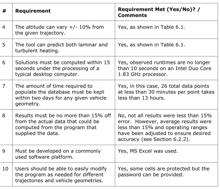
6.1.2 Verification of Requirements ... 44

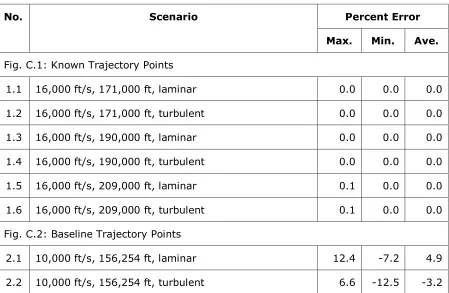
6.2 Results ... 45

6.2.1 Accuracy and Plots ... 46

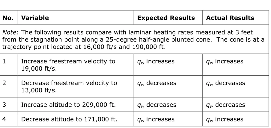
6.2.2 Observations and Discussion ... 51

Chapter 7 Conclusions and Recommendations... 55

7.1 Conclusions ... 55

7.2 Recommendations ... 55

References ... 58

Appendices ... 61

Appendix A - Cubic Spline Algorithm ... 62

Appendix B - xTRAPs Main Screen (Screenshot) ... 65

List of Tables

Table 4.1 - User Requirements ... 19

Table 6.1 - Functional Testing ... 43

Table 6.2 - Verification of Requirements ... 44

Table 6.3 - 25o _{Cone-half Angle Results ... 46}

Table 6.4 – 10o _{Cone-half Angle Results ... 48}

Table 6.5 - 45o _{Cone-half Angle Results ... 49}

Table 6.6 - Other Results ... 50

List of Figures

Figure 2.1 - Entry Corridor ... 5

Figure 2.3 - Deceleration and Heat Flux vs. Altitude ... 7

Figure 2.2 - Atmospheric Entry Trajectories on a Velocity-Altitude Map ... 7

Figure 2.4 - Heating Effects of Hypersonic Flow ... 10

Figure 5.1 - Baseline Trajectory with Deviation Limits ... 28

Figure 5.2 - Effects of Varying Cone-half Angle on Heating Rates Correlation ... 30

Figure 5.3 - Effects of Varying Altitude on Heating Rates Correlation ... 30

Figure 5.4 - Typical Velocity Correlation ... 33

Figure C.1 - 25o _{Results: Known Trajectory Points at V∞ = 16,000 ft/s ... 68}

Figure C.2 - 25o _{Results: Baseline Trajectory Points ... 69}

Figure C.3 - 25o _{Results: 10% Above Baseline Trajectory Points ... 70}

Figure C.4 - 25o _{Results: 10% Below Baseline Trajectory Points ... 71}

Figure D.1 - 10o _{Results: Known Trajectory Points at V} ∞ = 16,000 ft/s ... 73

Figure D.2 - 10o _{Results: 10% Above and Below Baseline Trajectory Points ... 74}

Figure E.1 - 45o _{Results: Known Trajectory Points at V} ∞ = 16,000 ft/s ... 76

Figure E.2 - 45o _{Results: 10% Above and Below Baseline Trajectory Points ... 77}

Figure F.1 - Other Results: Midrange Points, 35o _{Cone-Half Angle ... 79}

Figure F.2 - Other Results: Transition Point Examples (xt = 3.0 ft) ... 79

Figure F.3 - Other Results: Random Scenarios ... 79

Nomenclature

A constant dependent on angle-of-attack and geometry, unknown Alt altitude, ft

CD coefficient of drag, dimensionless

CL coefficient of lift, dimensionless

Cp specific heat capacity under constant pressure, ft-lb/(slugs-oR)

CFue correction factor for correlating velocity, dimensionless

g gravitational acceleration, ft/s2

g0 gravitational acceleration at sea-level, ft/s2

h enthalpy, ft-lb/slugs

haw adiabatic wall enthalpy, ft-lb/slugs

hcf heat transfer rate coefficient, slugs/(ft2-s)

hD diffusion enthalpy, ft-lb/slugs

L length of the body, ft

Le Lewis number, dimensionless

m mass, slugs

p pressure, lb/ft2

Pr Prandtl number, dimensionless q heat flux per unit area, BTU/(ft2_-s)

qc convective heat flux per unit area from gas to wall, BTU/(ft2-s)

qR radiative heat flux per unit area from gas to wall, BTU/(ft2-s)

qRS radiative heat flux per unit area from surface to gas, BTU/(ft2-s)

R gas constant, ft-lb/(slugs-o_R)

Rc radius of curvature, ft

RN nose radius, ft

r recovery factor, dimensionless S reference area, ft2

s distance along the surface of the body, ft

u velocity in the x-direction, ft/s V total velocity, ft/s

VE entry velocity, ft/s

x distance from leading edge, ft xT distance from transition point, ft

 angle-of-attack, degrees

 entry angle, degrees µ viscosity, lb-s/ft2

 running length from start of the streamline, ft ρ density, slugs/ft3

 Extrapolation factor, dimensionless

Subscripts

e at the edge of the boundary layer

L laminar flow

s at the stagnation point

T turbulent flow

w at the wall

0 total

1 known point in trajectory space

2 unknown point in trajectory space

Chapter 1

Introduction

The ability to accurately predict surface heating rates has proven to be one of the most significant issues to the design and development of planetary entry vehicles. This element as well as the shear and pressure forces used to calculate the aerodynamic behavior are fundamental to the analysis and design of the thermal protection system (TPS). The role of the TPS is to function as an effective insulator to protect the structure and payload of the spacecraft by ensuring, so called, burn-through of the outer wall of the vehicle does not occur due to the searing heat encountered during atmospheric entry. Proper TPS design is vital to prevent a possible disaster to planetary entry vehicles and crew. A common sited example is the disaster of Space Shuttle Columbia which occurred on February 1, 2003 when the orbital disintegrated during atmospheric entry due to hot-gases penetrating the wing structure resulting in the death of all seven crew members. Though the design of the TPS was not deemed at fault because the final accident investigation report determined that the TPS panel on the leading edge of the left wing was damaged from debris during launch1_{, it is an example of the grave} consequences that can exist without proper TPS insulation.

solely on full N-S solutions when considering the hundreds of trajectories and

geometries which are typical during the conceptual stage of the vehicle design process. Although Navier-Stokes solvers serve a significant role in detailed design analysis, the current focus is to develop accurate and more efficient approximate engineering codes to be used during preliminary or conceptual design. With an accurate definition of the aerothermodynamic environment, better estimates can be made of TPS weight and other properties earlier in the design process, which will improve the overall vehicle development.

1.1

Research Objectives

This research is to aid in the current efforts to develop new methods to rapidly compute convective heating rates on hypersonic vehicles done by H. H. Hamilton III and K. J. Weilmuenster of the Aerothermodynamic Branch of NASA Langley Research Center and Dr. F. R. DeJarnette of North Carolina State University. Previous work has largely been focused on developing more efficient inviscid and boundary layer approximate codes that when used in conjunction compare favorably with N-S calculations.

As a follow-up to the work done by these individuals, the NASA branch has requested that the findings of these programs be correlated to predict heating rates along the entire trajectory of a planetary entry vehicle. Although accurate boundary later code solvers, such as UNLATCH,3,4 _{have now been developed to rapidly compute heating rates} at a single trajectory point, it is still considered too time consuming to compute the large number of solutions required throughout the trajectory space when designing a

hypersonic vehicle. Therefore, the logical next progression to reduce the time to obtain the solutions is to construct the solutions using interpolation from a database of results previous computed. In this approach, known solutions are populated in a database for a particular vehicle shape and then the database is used to interpolate results that

approximate the CFD solutions at various other points in the defined trajectory space. This allows heating results to be predicted very quickly based on data calculated

interpolation it still requires a relative large number of database solutions. Since every time the vehicle configuration changes a new database is required to be generated, a much faster method to construct the approximate solutions is needed for preliminary design where the vehicle shape may undergo numerous changes.

1.2

Extrapolation Program

As presented in the report, a new approach to this problem has been developed which uses a combination of interpolation and extrapolation by utilizing boundary layer and hypersonic based correlations. When this new approach is combined with the use of an approximation method of solving the flowfield about a vehicle, such as with UNLATCH3,4_, then the database needed to construct the solutions can be populated within a few days using a relatively small number of known solutions in the database. Once the database is populated, this approach will give results within seconds of the heating rates at

Chapter 2

Background Theory

There are four critical parameters to consider when designing a vehicle for planetary entry - maximum heating rate, total heat load, maximum deceleration and maximum dynamic pressure. The maximum heating rate and maximum dynamic pressure

determine the type of TPS material while the total heat load influences the thickness of the insulating material. Maximum deceleration becomes a major factor for manned flight missions because human beings are limited by the amount of deceleration they can withstand over a certain amount of time.

2.1

Reentry Trajectories

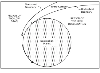
For manned reentry, it is important to safely define the overshoot boundary and

A vehicle in Low-Earth-Orbit (LEO), such as the Space Shuttle docked at the

International Space Station, will enter the Earth‟s atmosphere upon its return at speeds of approximately 7.9 km/s (25,919 ft/s, greater than Mach 25) – known as orbital or

satellite velocity. While bodies entering Earth‟s atmosphere from a lunar mission, such as one of the Apollo capsules, or an interplanetary mission, such as a possible return from Mars, will have entry speeds of 11.2 km/s (36,745 ft/s, greater than Mach 35) or more – known as escape velocity7_{. The Space Shuttle‟s body and large angle-of-attack} provide lift so it performs what is called a lifting or glide entry. However, the Apollo capsules had negligible lift so they performed what is called a ballistic entry and

essentially fall through the atmosphere under the influence of only drag and gravity (Fig. 2.2)7_{. In both cases, it is advantageous to use a blunt body vehicle to increase pressure} drag and naturally slow down the vehicle‟s velocity. However, as an even more

important benefit, the use of a blunt-nose body in flight above sonic velocity causes a detached bow shock wave to be formed ahead of the vehicle. This bow shock minimizes skin friction drag and thus deflects some of the hot gases from being in direct contact with the vehicle, resulting in reduced surface heating rates.

Destination Planet

Entry Corridor

Undershoot Boundary Overshoot

Boundary

REGION OF TOO LOW

DRAG REGION OF TOO HIGH

DECELERATION

As derived in various astronautical textbooks, the relationship relating freestream

velocity to density in a lifting and ballistic entry is shown below in Equations 2.1 and 2.2, respectively7_.

c

LS R

C m g V 1 2 1 2         _  (2.1)

 

Equation 2.1 is largely dependent on m/(CLS), called the lift parameter, which is related

to the geometry of the entry vehicle. The Rcin Equation 2.1 represents the radius of

curvature, which, in the case of entry to Earth‟s atmosphere, it is applicable to use the average radius of Earth (approx. 6.4e6 m or 2.09e7 ft)7_{. Likewise, Equation 2.2 is} largely dependent on m/(CDS),which is also a product of the geometry of the vehicle

but called the ballistic parameter. (Note: Equation 2.2 assumes an exponential model of the atmosphere to relate density to altitude.)

Figure 2.2 was created using Equations 2.1 and 2.2 with the lift and ballistic parameters listed in the legend. As shown, while penetrating the atmosphere at high altitudes the dominate effect of increasing density causes the deceleration to increase, but at lower altitudes the decrease in velocity dominates so the vehicle will reach a maximum

deceleration at a specific altitude. Likewise, the heating rate will reach a maximum at a specific altitude. This altitude will always be higher than the altitude of maximum

deceleration because heat flux is proportional to V∞3 while deceleration is proportional to

V∞2. As alluded to earlier, the maximum deceleration and maximum heating rates are

Figure 2.2 - Atmospheric Entry Trajectories on a Velocity-Altitude Map

2.2

Reentry Temperatures

A vehicle moving at hypersonic flight speeds will have a strong shock formed ahead of the body which converts most of the kinetic energy associated with the flight velocity into thermal and chemical energy8_{. Such is the case during direct planetary entry as} seen in the example of the Apollo capsule when the temperatures in the shock layer in the nose region of the vehicle reached 11,000 K during its return through Earth‟s atmosphere9_.

These extreme temperatures cause the atmospheric gases to no longer function as perfect gases with constant specific heats. The air that makes up the Earth‟s

atmosphere is primarily a binary mixture of nitrogen and oxygen10_{, but at typical reentry} velocities and temperatures the air compressed in the shock layer becomes both

dissociated and ionized. With increasing temperatures, higher energy modes are excited - molecules vibrate called vibrational excitation, break apart called dissociation and then

ionization occurs which is when electrons are released from the atoms leaving positive and negative charged ions. All of these real gas effects cause the air to stray from typically assumed perfect gas behavior and must be accounted for when analyzing the aerodynamic heating of a vehicle.

Since a reentry vehicle enters the atmosphere with such large kinetic and potential energy, which is primarily converted to heat during the descent, the priority during design is to deflect as much thermal energy as possible away from the vehicle in order to minimize the thermal energy that goes into the body.

2.3

Aerodynamic Heating

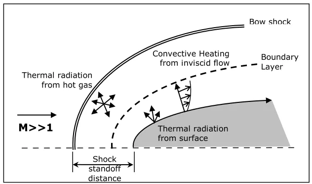
the flowfield around the body. Thermal radiation is not a significant source of

aerodynamic heating until the gas temperatures are high enough that the fluid elements radiate a substantial amount of energy. This threshold temperature for air is about 10,000 K9 _{which, as noted in Section 2.2, was reached in the shock layer in the nose} region of the Apollo capsule during its reentry to Earth. In this case, the thermal radiation accounted for more than 30% of the total aerodynamic heating to the body surface9 _{but, in the possible case of atmospheric entry to Jupiter, the thermal radiation} would account for more than 95% of the total heating. Since, this report focuses on atmospheric entry to Earth from LEO such as from the International Space Station, the effects of thermal radiation heating is beyond the scope of this document.

Convectional heating that occurs in the boundary-layer adjacent to the body as the vehicle passes through the surrounding atmosphere is due to frictional forces because the kinetic energy of the flow velocity is dissipated into internal energy, called viscous dissipation. However, this heating is compounded by what is known as shock-wave heating which occurs from the hot compressed gas ahead of the vehicle and behind the very strong shock that forms as a result from the extreme velocities reached during reentry9_{. Also, as a point of interest, as the wall temperature increases, there will be} thermal radiation from the wall surface as some of the heat will radiate away from the vehicle (Fig. 2.410_).

Therefore the heating rate at the wall, qw, can be calculated by the following equation:

RS R c

w q q q

q    (2.3)

M>>1

Convective Heating from inviscid flow Thermal radiation

from hot gas

Shock standoff distance

Bow shock

Thermal radiation from surface

Chapter 3

Aerothermodynamic Analysis

The hypersonic vehicle design process integrates experimental, numerical and analytical testing techniques along with flight tests data to analyze aerodynamic heating and properly define the aerothermodynamic environment present during a vehicle‟s flight mission. Only full-scale flight tests provide an actual representation of a vehicle‟s environment but, of course, this testing method is too expensive and impractical because it can only occur once extensive design has been completed2_{. Due to rising} costs and the inability of other methods to predict the aerothermodynamic environment, there is an increasing reliance on numerical, or rather, computational testing methods but this reliance does not diminish the importance of incorporating other testing methods. The following serves as a literary search sampling some of the various aerothermal analysis methods commonly used today.

3.1

Experimental Measurements

Experimental testing involves measuring data in a ground-based facility such as a wind tunnel, shock tube, arc-heated tunnel, ballistic range enclosure or on a sled rail test platform. Since no one facility can simultaneously simulate the higher Mach numbers and high flowfield temperatures of the hypersonic flight environment12_{, various facilities} are used to test different aspects of hypersonic flight. For instance, to simulate altitude in a wind tunnel, a freestream static pressure is chosen that corresponds to the pressure at a given altitude for standard atmosphere9_{. However, the freestream static}

but, as in some cases, it is lowered to decrease the speed-of-sound and simulate an increase in the freestream Mach number. Although, these methods are effective to achieve their desired specific result, they do not simultaneously simulate the

environment of flight. However, when used in collaboration, ground-based testing can adequately obtain aerodynamic forces and moments, pressure distributions and predict the heat transfer distributions.

Compared to computational testing, the time required to fabricating models and conducting various test procedures can make experimental testing time and cost inefficient. However, experimental testing still serves a vital role in modern aerothermodynamics because experimental testing is used complementary to

computational testing to provide data to develop realistic computational flow models and then validate, calibrate and compare results obtained from developed computer codes.

3.2

Numerical Solutions

many detailed computational codes are the complex geometries and long run-times required to execute the solutions.

Various computer codes have been developed to calculate radiative and convective heating rates. However, due to the focus of this report, only some of the convective heating codes are summarized below.

3.2.1

Navier-Stokes Code Solvers

Full Navier-Stokes (N-S) code solvers provide the most accurate detailed solutions of surface heating rates of hypersonic reentry vehicles as validated based on measured flight data. Therefore, their ability to accurately predict aerothermal loading has proved to be an invaluable resource to the design of thermal protection systems.

One such N-S solver is the Langley Aerothermodynamic Upwind Relaxation Algorithm (LAURA) which has been used as a benchmark to validate various other code solvers and experimental testing methods. LAURA is a structured, multi-block, computational

aerothermodynamic simulation code that uses a finite-volume approach to solve the inviscid, thin-layer Navier-Stokes, or full Navier-Stokes flowfield equations13_.

Detailed N-S solvers require considerable computer storage requirements and long run-times so they are often a too expensive form of testing. For a typical reentry vehicle configuration most N-S solvers compute tens-of-million calculations to obtain a solution. As expected, this magnitude of calculations requires a large cluster of processing

workstations and still results in run-times typical of 1-3 weeks to obtain a single

solution. Time and resources cost money, so full N-S solvers should only be used when accuracy is most critical.

3.2.2

Approximate Boundary Layer Solutions

Effective BL code solvers implement applicable hypersonic approximations to the equations that govern fluid flow to reduce their computation time while minimizing the loss in accuracy. These viscous codes use boundary layer theory formulas which first require the inviscid solution to be computed to determine the boundary layer edge conditions required to complete the viscous calculations. Various BL codes have been developed to function in conjunction with the various developed inviscid flow solvers.

SABLE:

SABLE is a finite-difference code for laminar or turbulent boundary layer solutions over axisymmetric bodies developed in 199214_{. It can compute solutions using ideal gas,} carbon tetrafluoride (CF4) or equilibrium air chemistry. SABLE computes boundary layer solutions within seconds that compare favorably with N-S solutions, but its limitation is that it must work in conjunction with a structured grid generated inviscid flow solver.

One such structured grid inviscid code is BLUNT2D which is a time-dependent solution for axisymmetric flow over a blunt body that was developed by H. Harris Hamilton and John R. Spall in 198615_{. The typical run-times of BLUNT2D are on the order of a few} minutes.

LATCH and UNLATCH:

Langley Approximate Three-dimensional Convective Heating (LATCH) code was

developed to compute viscous solutions using single block structured grids16,17_{. As an} extension to this code using unstructured grids, Hamilton et al. created a viscous code solver called UNLATCH that, when used in conjunction with a full three-dimensional, inviscid flowfield solution, rapidly computes convective heating rates that compare with N-S solutions3,4_.

LATCH and UNLATCH are based on the axisymmetric analog for general

three-dimensional layer equations to the same form as the axisymmetric boundary-layer equations18_{. Therefore, the heating on a three-dimensional body is computed} along inviscid surface streamlines by replacing the radius of the axisymmetric body with the metric coefficient that is related to the converging or diverging of the surface

streamlines. UNLATCH is also capable of computing finite catalytic wall effects on heating using an approximate method developed by Dr. George Inger19_.

One such inviscid flow solver commonly used in conjunction with UNLATCH is CART3D, which is a finite volume based flow solver originally created for subsonic/transonic flight regime, but has since been extended to the hypersonic flight regime16_{. Using these} applications, a typical solution for both laminar and turbulent flow can be computed in approximately 15-30 minutes, depending on the complexity of the vehicle‟s mesh.

3.2.3

Interpolation Programs

Grant Palmer has developed a program titled Automated Design Space Interpolation (ADSI) code to interpolate a database of surface solutions to a point in the trajectory space5,6_{. ADSI performs a series of complex interpolation schemes in a one-, two-, or} three-dimensional trajectory space. Once the database is populated, ADSI performs very efficient calculations with acceptable accuracy. However, ADSI requires a fair number of database solutions and does not consider mathematical relationships that exist between the interpolated variables.

3.3

Analytical Solutions

3.3.1

Fay and Riddell

In 1957, Fay and Riddell20 _{carried out a rigorous study of stagnation heat transfer, q}

w,s,

at hypersonic speeds which resulted in the following expression for equilibrium boundary layer:



 











w 0.57 ₃4 Pr ρ μ ρ μ du_dx h h 1 Le 1 h_h

q (3.1)

where: j=0 for two-dimensional flow and j=1 for axisymmetric flow.

The term in the square bracket, which accounts for the contribution of chemical reactions, is approximately 1.0 for binary mixtures, such as air, so it can safely be neglected in preliminary analysis10_{. As noted by Anderson}9_{, Fay and Riddell‟s analysis} covered a range of velocities from 5800 to 22,800 ft/s and wall temperatures from 300 to 3000 K (540 to 5400 o_{R). Remarkably, Fay and Riddell‟s equation is still considered} today to be the most accurate method to calculate the stagnation heat transfer rate.

Another similar equation given by Van Driest in 195621 _{prior to Fay and Riddell is the} following.









. 0 s

,

w _dx h h

du μ ρ Pr 763 . 0

q _ 

    

  _(3.2)

Equation 3.2 applies to the stagnation point of a sphere in equilibrium. It is similar to the axisymmetric version of Fay and Riddell‟s equation except it does not account for chemical reactions and the often difficult to predict density and viscosity wall properties are not required.

3.3.2

Generalized Heating Equations

flat-plate at an angle-of-attack22_{. These heating equations take the form of the} following expression9_:

C V ρ

q_w  _N _M (3.3)

where: N & S – exponential constants

C – constant specific to geometry

The coefficients in Equation 3.3 are given as the following. (Note: the C values are derived to work only with SI base units, and the resultant units of qw are W/cm2.)

Stagnation point flow:

              0 5 . 0 ₁ 8 83 . 1 3 5 . 0 h h R e C M N w N (3.4)

Laminar flow over a flat plate:





0 _{sin( ) 1}

) cos( 9 53 . 2 2 . 3 5 . 0 h h x e C M N w   (3.5)

Turbulent flow over a flat plate:



 



1 _{1 1.11}

556 ) sin( ) cos( 8 89 . 3 37 . 3 / 3962 : with 8 . 0 h h T x e C M s m V N w w T   (3.6)



 



2 _{sin( ) 1 1.11}

Additionally, there is an alternative value for the coefficient of C in Equation 3.4 to calculate the heating rating in Earth‟s atmosphere given by Sutton-Graves23 _that assumes hw/h0 <<1, the so called very cold wall approximation:

5 . 0

8 74153 .

1 _{ } 

 e R_N

Chapter 4

Requirements and Considerations

When developing xTRAP, it was advantageous to follow the engineering design process of first defining user requirements and then outlining conceptual design considerations.

4.1

Requirements

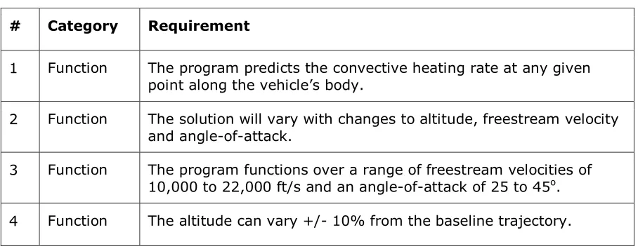
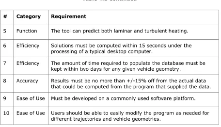
The objective is to develop a program that that can rapidly predict convective heating rates at a given point along a transatmospheric trajectory over the entire surface of a vehicle which will be beneficial to the preliminary design of reentry vehicles. In order to meet this objective the following user requirements were developed and categorized under the main concerns of function, accuracy, efficiency and ease of use (Table 4.1).

Table 4.1 - User Requirements

# Category Requirement

1 Function The program predicts the convective heating rate at any given point along the vehicle‟s body.

2 Function The solution will vary with changes to altitude, freestream velocity and angle-of-attack.

Table 4.1 Continued

# Category Requirement

5 Function The tool can predict both laminar and turbulent heating.

6 Efficiency Solutions must be computed within 15 seconds under the processing of a typical desktop computer.

7 Efficiency The amount of time required to populate the database must be kept within two days for any given vehicle geometry.

8 Accuracy Results must be no more than +/-15% off from the actual data that could be computed from the program that supplied the data. 9 Ease of Use Must be developed on a commonly used software platform.

10 Ease of Use Users should be able to easily modify the program as needed for different trajectories and vehicle geometries.

4.1.1

Function

The purpose of developing this program is to predict convective heating rates over the surface of a vehicle during a reentry trajectory. Interpolation will occur among known data points varying with altitude, freestream velocity and angle-of-attack. Therefore, the database tool must show the effects of changing the altitude, freestream velocity or angle-of-attack has on the resultant predicted heating rates.

4.1.2

Efficiency

This program is being developed to aid in the preliminary design process of thermal protection systems. Therefore, the time required to compute the solution is essential and the accuracy of the results can be sacrificed to promote the efficiency. The

efficiency is dependent on both the time required to populate the database and the time to execute the solution once the database has been populated. Both of these elements must be kept at a minimum to be a useful preliminary design tool.

In order to minimize the amount of time to populate the database, it is important to investigate what is the minimum number of known data points required to achieve the required accuracy (See Section 4.1.3). Since of the majority of the time required to compute a solution will be consumed by first populating the database, keeping this number of known data points to a minimum will have the largest effect on efficiency. Once the database has been populated for a given vehicle‟s geometry then locations throughout the trajectory space can be selected to predict the new data without the need to re-populate the database. Therefore, reducing the time required to execute the solution (User Requirement #6) is also a concern.

4.1.3

Accuracy

The tool is only as accurate as the supplied data used to populate the database. If the supplied data is poor, then the extrapolated solutions will be poor, but if the supplied data is reasonably accurate then the resultant extrapolated data should be sufficiently accurate. If accuracy is the main concern, then the database can be populated with solutions given by Navier-Stokes code based solvers. However, since this is to be used during preliminary design, it is more practical to use a boundary layer solver that has shorter runtimes to calculate the heating rates to populate the database such as SABLE or UNLATCH (see Section 3.2.2).

have no more than 15% error. Critical locations throughout the flowfield will be chosen to compare the percent error between the predicted value resulting from this tool and the actual value that could be calculated using the program that generated the supplied data.

4.1.4

Ease of Use

In order for this tool to be regularly utilized, it must be user friendly and adaptable for many different applications. The database tool must be developed on a common software platform such as Microsoft Excel or Microsoft Assess making it easy to share among users. The tool will be protected to ensure regular users do not make a change that is detrimental to the program but the password will be provided to allow advanced users to make changes as necessary. The user will be able to modify the baseline trajectory and supplied source data for different vehicle‟s geometry as needed.

4.2

Design Considerations

4.2.1

Trajectory and Geometry

The baseline trajectory for this program should be chosen to represent a typical reentry trajectory of a vehicle similar to design and mission of the Space Shuttle. A typical mission of the Shuttle or any similar replacement vehicle would be to fly to the

International Space Station in Low-Earth-Orbit (LEO), complete various experiments and then return safely to Earth. As mentioned in Section 2.1, the Shuttle performs a lifting entry with the velocity varying with altitude represented by Equation 2.1. However, the vehicles proposed to replace the Shuttle have geometries similar to the Apollo capsules so, their associated lift parameter would be higher than the Shuttle but they are

expected to still perform a lifting entry. Therefore, for the purpose of this program, the standard atmosphere data, along with a lifting entry and a relatively high lift parameter, will be chosen to determine the baseline trajectory.

The geometry chosen for the entry vehicle of this program will be a blunt-nose body typical of many reentry vehicles. To simplify the program, an axisymmetric spherical nose cone is chosen so specific locations along the body can be defined by their surface distance from the nose.

4.2.2

Number of Data Points

As alluded to in Section 4.1.2, an important question that must be answered is how many data points will need to be calculated to populate the database and ensure

4.2.3

Interpolation

By definition, interpolation is a method of constructing new data points within the range of a discrete set of known data points. In general, the process of determining a function that closely fits known data points is called curve fitting or regression analysis.

However, the drawback with implementing a regression fit over multiple data points is that the determined trend line does not necessary pass through the known points. However, interpolation is a specific type of curve fitting that ensures that the function goes exactly through the data points.

Linear Interpolation

The simplest form of interpolation is linear interpolation which assumes a straight line approximation between adjacent data points. Given two data points, (xa,ya) and (xb,yb),

the linear interpolation relation is given by:

) ( ) ( ) ( a b a a b

a y y _xx x_x

y y    

 at the point (x,y) (4.1)

The limitation of linear interpolation is that it is not very precise or smooth because it is piecewise linear and only depends on the adjacent data points, so knowing values of additional points do not improve the accuracy of the approximation.

Polynomial Interpolation

Polynomial interpolation is an extension of linear interpolation because it seeks to fit a higher order polynomial to the data points. Polynomial expressions of the following form are used to interpolate a value at point (x,f(x)) with coefficients A, B, C, D, etc.

representing curve fitting constants:

... )

(x A Bx Cx2 Dx4

f     (4.2)

tends to be a more complicated solution and it has the potential to create unwanted oscillations.

Spline Interpolation

Spline interpolation is similar to linear interpolation in that it creates piecewise segments between each adjacent data points but it typically fits low-order polynomial functions as opposed to linear piecewise functions. What makes spline interpolation unique is that the chosen low-order polynomial segments are several times differentiable so the

solution is smooth and the unwanted oscillations of higher-order polynomial interpolation are eliminated26_{. Spline interpolation is more difficult to compute than simple linear} interpolation, but it is often easier to compute than high-order polynomial interpolation.

From a practical point of view, cubic splines are most commonly implemented. A cubic spline is a continuous function that has continuous first and second derivatives

everywhere in the interval and in each subinterval of the partition, and is represented by a polynomial of degree three26_.

4.2.4

Extrapolation

Another important element to understand when developing this program is the concept of extrapolation. Extrapolation is a method to construct data points outside a discrete set of known data points. Compared to interpolation, extrapolation can be rather uncertain because it projects data past the boundaries of known data points.

Extrapolation assumes that a similar relation exists outside the data points as observed between the data points. Extrapolation methods can be linear, polynomial, spline, etc. but the use of polynomial or spline extrapolation can often cause large spikes in

approximations so caution must be used when applying relations outside of known data points.

Extrapolation methods can become less risky if proven physics based expressions are used to project the data. In the case of this task, proven hypersonic approximations and boundary layer expressions will be used where appropriate to reduce the

Chapter 5

Analysis and Design

This chapter details the procedure used to develop xTRAP and summarizes the final design.

5.1

Analysis

5.1.1

Extrapolation Procedure

xTRAP follows a procedure, as advised from H. Harris Hamilton, to approximate the convective heating rates in trajectory space24_{. As previously mentioned, this procedure} is adapted from a method used by Dr. R. Merski to extrapolate surface heating rates from a wind tunnel test model to flight conditions25_{. This procedure is applicable to} approximate the surface heating rate in trajectory space for a single point on a three-dimensional body at an angle-of-attack. However, to simplify the description and the computational time required to generate source data, the procedure has been applied to an axisymmetric spherically blunted cone at zero angle-of-attack. As such, different cone half-angles will replace angles-of-attack in this analysis and discussion because changing either of these elements has the same effect on the heating along a body24_.

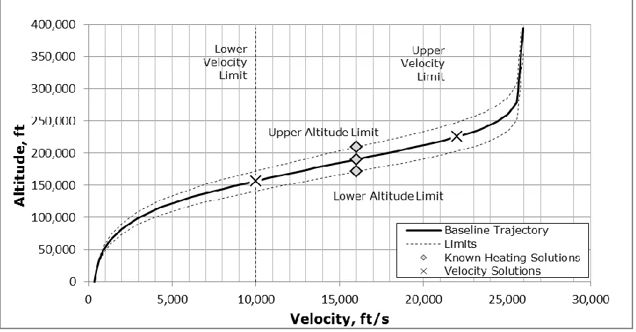
Assume the cone enters an atmosphere on the lifting entry trajectory shown in Figure 5.1. If a database of known solutions consist of the following:

1. Heating solutions computed at the mid-freestream velocity over a range of cone half-angles, on the baseline trajectory and at specified altitudes above and below the baseline altitude (indicated by diamond shape in Fig. 5.1), and

2. Inviscid velocity solutions computed at regular intervals along the baseline trajectory (indicated by „X‟ in Fig. 5.1).

Then, the following procedure can be used to extrapolate heating solutions to various other points within the defined trajectory space shown.

(lift parameter = 733 kg/m2 _{(4.67 slugs/ft}2₎₎

The extrapolation procedure relies on the following principle which relates the heat transfer coefficient for a position along the body to the heat transfer coefficient at the stagnation point for laminar flow:



s , cf

cf

h h

constant (5.1)

This statement is valid because both hcfand hcf,s have the same functional dependence

on Reynolds number24_{. Mathematically, Equation 5.1 can also be expressed by the} following equation comparing Point 2 to Point 1 in the trajectory space with 

representing an extrapolation factor.

 1 s , cf cf 2 s , cf cf h h h h                  (5.2)

From Equation 5.2, if the heat transfer coefficients are known at Point 1 ([hcf /hcf,s]1) and

the stagnation point heat transfer coefficient can be calculated at Point 2 (hcf,s,2), then

the following equation can be used to calculate the heat transfer coefficient at Point 2 (hcf,2) if an appropriate  value is determined.

 1 s , cf cf 2 , s , cf 2 ,

cf h _hh

h          (5.3)

(Note: Adding the  value expands this formula to be used for turbulent flow

extrapolations, see Section 5.1.4) Then, from knowing the value of hcf,2, the heating

rate at the wall, qw,2 can be determined by the following equation:





2 , cf 2 ,

w h h h

q   (5.4)

This is the basic method of extrapolation used to develop xTRAP. However, the following details are needed to understand how to utilize these equations.

5.1.2

Known and Unknown Points

The database solutions computed at the midway point of the freestream velocity range (at V∞=16,000 in Figure 5.1) are represented by the subscript 1. These solutions share

trajectory space where the solution is not yet known. Point 1 values are interpolated based on values specified by the user for Point 2‟s configuration and location before the data is extrapolated to a new location. Specifically, the user specified angle-of-attack determines the appropriate cone-half angle solution to be used at Point 1 and the altitude specified by the user for Point 2 determines the percent above or below the baseline altitude used for Point 1.

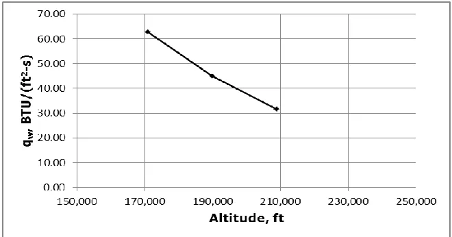
The following figures show how the heating rate changes with cone-half angle and altitude, respectively (Fig. 5.2 and 5.3).

Figure 5.2 - Effects of Varying Cone-half Angle on Heating Rates Correlation

5.1.3

Extrapolation Terms

Instead of working with heating rates, qw,directly, this procedure deals with heat

transfer coefficients because heat transfer coefficients are relatively insensitive to wall temperature24_{. The following defines the heat transfer coefficient:}





cf _h q _h

h



 (5.5)

The adiabatic wall enthalpy, haw, is calculated by the following:

          2 u r h

h e2

e

aw (5.6)

where r is the recovery factor which is approximately equal to the following for laminar and turbulent flow, respectively.

r_L  Pr (5.7)

3

T Pr

r  (5.8)

The wall enthalpy, hw, is determined based on knowing the thermodynamic properties at

the wall. In the case of computing solutions using the boundary layer code SABLE (see Section 3.2.2), the wall temperature and pressure at the edge of the boundary layer are given in the outputted data file. If the database solutions are computed for perfect gas then the following equation can be used to calculate wall enthalpy.

h_w C_pT_w (5.9)

However, if the database solutions are computed for equilibrium air chemistry, such as used in xTRAP, one must look-up the wall enthalpy based on knowing two

thermodynamic properties (Twand pe) because the pressure does not change in the

p_w  p_e (5.10)

In order to apply Equation 5.4, Equation 5.6 is used to determine haw and two

thermodynamic properties are used to determine hw. However, the local properties at

the edge of the boundary layer are first needed to determine he in Equation 5.6 and to

determine one of the wall properties based on Equation 5.10. The non-dimensional ratio of the boundary layer edge pressure to the freestream dynamic pressure has been found to correlate the local pressure reasonably well (Eq. 5.11).

               2 e V ρ 2 1 p constant (5.11)

Therefore, the edge pressure can be approximated by the following:





p _

           (5.12)

When determining the ue term in Equation 5.6, it was noted that a non-dimensional

velocity term (ue2/V∞2) does not correlate like the pressure. Therefore, a correction

factor for the velocity, CFue, can be added for the correlation in the following form:

_ue 1 2 e 2 e 2 2 , 2 , e CF V u V

u _

     

 _ (5.13)

The correction factor, CFue, can be determined by interpolating the non-dimensional

Once the edge velocity is calculated, the edge enthalpy is calculated from Equation 5.14 with the total enthalpy defined in Equation 5.15.

2 u h

h e2

2 , 0 2 ,

e   (5.14)

2 u h h₀ 2

 

 (5.15)

Now both pe and he are known so other thermodynamic properties such as Teand e can

be looked up in equilibrium air tables.

The only remaining Point 2 parameter needed to apply Equation 5.4 is a value for the wall temperature. If Tw,2 was known, then hw,2 of Equation 5.4 can be determined by

looking up in equilibrium air tables since pw,2 is already known. However, if Tw,2 is not

known, the radiative equilibrium wall condition can be applied to solve this temperature. This is a condition when the convective heat transfer to the wall is equal to the radiative heat transfer away from the wall, represented in the following equation:

q_w q_RS (5.16)

The radiative surface heat transfer rate, qRS, is defined by the following formula, with ε

representing thesurface emissivity (approximated at 0.9) and  the Stefan-Boltzmann constant (4.761e-13 BTU/(ft2_-s-o_R4_):

4

w

RS T

q  (5.17)

Then, set the right side of Equation 5.4 equal to the right side of Equation 4.16 and solve for Tw,2 as shown below:

h_cf,2





Since hw,2 is dependent of Twthis equation must be solved iteratively. Once this value

is solved, everything required to complete the extrapolation is known, assuming the stagnation heating rate can be calculated, and an appropriate value for the extrapolation factors can be approximated for both laminar and turbulent flow.

5.1.4

Stagnation Heating

Fay and Riddell‟s equation (Eq. 3.1) was chosen to determine the stagnation heating rates, qw,s, for Point 1 and Point 2 which were then converted to heat transfer

coefficients based on Equation 5.5. Simpler methods such as Van Driest‟s equation (Eq. 3.2) and Sutton-Graves‟ generalized equation (Eq. 3.8) were also used in developing xTRAP, but, as expected, the Fay and Riddell method proved to be most accurate. The

due/dx term in Equation 3.1 was obtained from the modified Newtonian theory as the

following:





1

e e N

e 2p p

R 1 dx du

   



 

 

Therefore, the Fay and Riddell formula took the following form:



 







The total enthalpy was calculated from Equation 5.15 and the nose radius was given by the cone‟s geometry. The density at the edge of the boundary layer was determined by looking in equilibrium air tables and knowing the edge pressureandenthalpy from Equation 5.12 and 5.14, respectively. The wall enthalpy and density was looked up in equilibrium tables after iteratively determining the wall temperate from Equation 5.18 and knowing the wall pressure from Equation 5.10. The edge and wall viscosities shown in Equation 5.20 were calculated based on Sutherland’s Law9_{. Sutherland‟s Law says for}

a pure, non-reacting gas, the viscosity coefficient is dependent only on temperature by the following relationship:

_               S T S T T

T 2 ref 3 ref ref   (5.21)

Where28_:

K 6 . 110 S K 1 . 273 T s m / kg 5 e 789 . 1 ref ref     

5.1.5

Extrapolation Factors

As implied in Section 5.1.1 the extrapolation factor of Equation 5.3 is approximately equal to unity for laminar flow. However, the extrapolation factor for turbulent flow is not as simple. Merski looked at heat transfer rate correlations reported by Tauber and Meneses22 _{to develop his extrapolation factors to relate his wind tunnel model data to} flight conditions25_{. These derivations are outlined below and they form the basis for the} extrapolation values implemented in xTRAP.

0 s 5 . 0 5 . 0 c 3 5 . 0 s , cf _h A L L R V

h  

       

  (5.22)

where L is the length of the geometry and A is a constant dependent on angle-of-attack and geometry considerations. Likewise, the heat transfer coefficient for a laminar flat-plate is the following:

0 L 5 . 0 5 . 0 2 . 3 5 . 0 L , cf _h A L L V h          

   (5.23)

where is the running length from the start of the streamline. For turbulent flow, Merski listed the following correlation:

0 T 25 . 0 w 2 . 0 2 . 0 37 . 3 8 . 0 T , cf _h A T L L ξ V ρ

h   

         (5.24)

where is the running length from the start of transition. However, according to the other form of the generalized heating equation for turbulent flow, given in Section 3.3.2 (Eq. 3.7), an alternative form of the heat transfer coefficient for turbulent flow can be derived as the following:

0 T 2 . 0 2 . 0 7 . 3 8 . 0 T ,

cf ρ V ξ_L L _hA

h  

         (5.25)

Based on these correlations, extrapolation factors for laminar and turbulent flow can now be determined by dividing the local laminar or turbulent enthalpy, hcf (Eq. 5.23 and

5.24/5.25, respectively)by the stagnation point enthalpy, hcf,s (Eq. 5.20). From

1 s , cf L , cf 2 s , cf L , cf L h h h h                   (5.26) 1 s , cf T , cf 2 s , cf T , cf T h h h h                   (5.27)

So, if Equations 5.22, 5.23, 5.24 and 5.25 are substituted into Equations 5.26 and 5.27 and cancelations are made for running lengths, , and the constants, A, the

extrapolation factors result in the following:

2 . 0 1 , 2 , L _V V             (5.28) 25 . 0 1 , w 2 , w 3 . 0 1 2 37 . 0 1 , 2 , 3 . 0 1 , 2 , T _T T L L V V ρ ρ Χ                                     (5.29) 3 . 0 1 2 7 . 0 1 , 2 , 3 . 0 1 , 2 ,

T _V L_L

V ρ ρ Χ _                           _(5.30)

As said, the laminar extrapolation factor is approximately unity, but the value given in Equation 5.28 was preferred in developing xTRAP because it was found to give better results. According to the freestream velocity associated with Equation 3.7, the turbulent extrapolation factor derived by Merski in Equation 5.29 would best apply when

xTRAP. xTRAP does have the ability to extrapolate parameters to freestream velocities below 13,000 ft/s but Equation 5.30 was still found to give better results than Equation 5.29 because the dominating effects of Point 1.

The turbulent extrapolation factors are somewhat more complicated than the laminar results, but based on results of xTRAP, Equation 5.30 has been simplified to the following: 7 . 0 1 , 2 , 3 . 0 1 , 2 , T _V V ρ ρ Χ _                    _(5.31)

Dropping the ratio of geometry length, L, in Equation 5.30 can easily be justified for the case of xTRAP because the size and shape of the vehicle‟s body does not change

between Point 1 and Point 2.

5.2

Design

The following information details the design of the various components of xTRAP.

5.2.1

Database and CFD Solutions

In order to easily store and manipulate large amounts of heating data, Microsoft (MS) Excel was chosen to develop this extrapolation tool. Recent versions of MS Excel do not have the data restrictions of previous versions and it provides many numerical analysis functions that are not as easily implemented using a database program such as

Microsoft Access. Microsoft Excel was also chosen because it is well known in industry and it allows algorithms, such as cubic splines algorithms, to be easily added for interpolation applications.

than perfect gas assumptions in the range of Mach numbers considered (approximately Mach 10 to Mach 22). After running the BLUNT2D inviscid solution the SABLE code was run for both laminar and turbulent flow, and the data from the output file were copied as text into the MS Excel database.

5.2.2

Trajectory and Geometry

The baseline trajectory was calculated by listing U.S. Standard Atmosphere, 197629 _data at 5000 meter altitude increments from 0 to 40 km and 80 to 120 km and 1000 meter increments from 40 to 80 km. The atmospheric densities were then used in the lifting entry equation (Eq. 2.1) with a radius of curvature of 6.39e6 meters and a lift parameter of 733 kg/m2_{. These numbers can be adjusted as needed but were chosen to represent} a lifting body entry vehicle returning from LEO with a lift-to-drag ratio lower than the Space Shuttle.

As advised, a blunted sphere nose cone was used for the vehicle‟s body. The cone has a one-to-seven ratio of nose radius to body length. The results were analyzed based on a nose radius of 2 feet and body length of 14 feet. The cone-half angle ranged from 10 to 45 degrees to analyze the effects of changing angle-of-attack. The solutions computed along the baseline trajectory were at a cone-half angle of 25 degrees which is near midway between the angles of interest.

5.2.3

Interpolation and Extrapolation

A Visual Basics Application algorithm (Appendix A) was written based on common codes available on the internet and added to the Excel program to determine cubic spline interpolation. Once the algorithm was added, the implementation of cubic splines was actually easier than basic linear interpolation, so the use of cubic spline interpolation is preferred anytime the curve fit would be perceived different from a linear function. Therefore, cubic splines are utilized when reading the SABLE output data and when interpolating between cone-half angles, altitudes and velocities. The only time a linear interpolation method is utilized is when the program interpolates freestream

isothermal or gradient temperatures regions, which are piecewise linear segments characteristic of linear interpolation.

Extrapolation methods are used to project results from 16,000 ft/s to other points within the defined trajectory space. However, the observed trend data between known points are not simply extended to other points outside the known data points. Instead, the heating data is extrapolated based on known hypersonic and boundary layer theory as detailed in Section 5.1.

5.2.4

Number of Data Points

The following data points were computed and stored in the database in order to analyze the accuracy over the range of freestream velocities specified in Table 4.1 (10,000 to 22,000 ft/s). Four data points at cone-half angles 10o_{, 15}o_{, 25}o _{and 45}o _{were computed} on the baseline at 16,000 ft/s to account for changing angle-of-attack. To improve the results when the vehicle strayed higher or lower than the baseline trajectory, four data points were also computed at angles 10o_{, 15}o_{, 25}o _{and 45}o _{at 10% higher than the} baseline altitude at 16,000 ft/s and four more points were computed at angles 10o_{, 15}o_, 25o _{and 45}o _{at 10% lower than the baseline altitude at 16,000 ft/s. Two additional 25}o cone-half angle data points at 10,000 and 22,000 ft/s along the baseline trajectory were computed to correlate velocities. Including both laminar and turbulent solutions at each of the data points at 16,000 ft/s, but not along the other baseline points, made the total number of data points equal 26.