An integrative probabilistic model for identification of structural variation in sequencing data

M E T H O D

Open Access

An integrative probabilistic model for identification

of structural variation in sequencing data

Suzanne S Sindi

, Selim Önal

, Luke C Peng

, Hsin-Ta Wu

and Benjamin J Raphael

Abstract

Paired-end sequencing is a common approach for identifying structural variation (SV) in genomes. Discrepancies between the observed and expected alignments indicate potential SVs. Most SV detection algorithms use only one of the possible signals and ignore reads with multiple alignments. This results in reduced sensitivity to detect SVs, especially in repetitive regions. We introduce GASVPro, an algorithm combining both paired read and read depth signals into a probabilistic model that can analyze multiple alignments of reads. GASVPro outperforms existing methods with a 50 to 90% improvement in specificity on deletions and a 50% improvement on inversions. GASVPro is available at http://compbio.cs.brown.edu/software.

Background

Structural variation, including duplications, deletions and rearrangements of large blocks of DNA sequence, is now recognized as an important contributor to the genetic differences between individual humans and the somatic differences between normal and cancer cells [1-7]. It is also prevalent in other organisms, including many model organisms [8-10]. Knowledge about the extent of structural variation has increased rapidly in the past few years with improvements in DNA microar-ray and sequencing technologies. In particular, sequen-cing approaches identify all types of structural variation, including copy number variants and balanced rearrange-ments like inversions and reciprocal translocations [11-13]. While next generation sequencing technologies are now widely used to assess both genetic variation in normal genomes [14-21] and somatic structural varia-tion in cancer genomes [4,7,22,23], the short reads and short inserts of these technologies make the identifica-tion of many structural variants (SVs) non-trivial. Since de novo assembly of mammalian genomes from next-generation sequencing technologies remains a challenge [24,25], many SVs are identified using a resequencing approach where sequence reads from an individual gen-ome are aligned to a reference human gengen-ome assembly. The resequencing approach thus leverages the extensive

finishing efforts employed in the generation of the human reference genome.

Many strategies have been employed to predict struc-tural variation using the resequencing approach [11-13]. First, read depth (RD), the density of mapped reads to an interval of the reference genome, has been used success-fully to identify copy number variants [26-31]. However, RD is unable to detect copy neutral variants such as inversions and balanced translocations. Second, paired read (PR) approaches have been used to identify all types of SVs, both copy number variants and copy-neutral var-iants [16,28,32-35]. These approaches analyze the collec-tion of PR mappings and find clusters of aberrantly mapped PRs that suggest SVs distinguishing the two gen-omes. Third, split read (SR) methods have been employed to directly identify sequence reads that contain breakpoints of SVs [36]. However, the short reads pro-duced by current second-generation sequencing technol-ogies have limited the use of SRs for SV detection; for example, Yeet al. [36] rely on anchoring the search for SRs using a full-length alignment of one read from a PR.

While there has been extensive development of meth-ods for structural variation prediction, there remains room for improvement. First, most existing methods for SV prediction use only one of the possible signals (RD, PR or SR). A few methods employ a second signal in later post-processing of predictions. Such a post hoc approach may improve specificity, but it does not increase sensitivity by combining multiple, weak signals. Although a few recent methods have begun to consider both RD

* Correspondence: [email protected]; [email protected] 1

Center for Computational Molecular Biology, Brown University, Box 1910, Providence, RI 02912, USA

Full list of author information is available at the end of the article

and PR signals [37,38], these methods have focused only on copy number variants. Second, most methods for struc-tural variation prediction used only reads with unique high-confidence alignments to the reference genome, ignoring reads with lower quality alignments or multiple possible alignments [32,33,39]. As such, these methods have very low sensitivity to detect repeat-associated rear-rangements. Since many SVs are associated with repetitive sequences, including segmental duplications [40], and mobile elements [2], a substantial improvement in sensi-tivity may be possible by including reads with multiple alignments. More recently, a few methods have been intro-duced that consider multiple or lower quality alignments of reads relying on various criteria to select among possi-ble candidate alignments [34,41,42]. While these methods may predict more true variants, this increased sensitivity often comes at the cost of reduced specificity as these methods produce many false positive predictions. Thus, there is a need for additional improvements in sensitivity and specificity for SV prediction. For example, the pilot study of the 1000 Genomes Project did not report inver-sion SVs [43] even though such variants have been pre-viously shown to be abundant in normal genomes [16].

Here, we introduce GASVPro, an algorithm for SV iden-tification that integrates both RD and PR signals into a unified probabilistic model. We find that the likelihood of a predicted variant under our probabilistic model provides a better criteria for prioritizing predictions than the num-ber of supporting PRs, a common heuristic for ranking predictions. In addition to combining both RD and PR sig-nals, GASVPro explicitly reports uncertainty in each pre-dicted breakpoint, which is useful information for identification of SRs or designing assays for experimental validation. This breakpoint localization is obtained using a computational geometric algorithm, Geometric Analysis of Structural Variants (GASV) [33], that represents all pos-sible breakpoints, or breakends, that are consistent with the aligned reads as a polygon in two-dimensional genome space. By carefully clustering only those PRs that genuinely support the same breakends, GASV avoids over-collapsing fragments into the same SV prediction, a problem demon-strated in other methods (see Results) and reports coordi-nates consistent with the true variant points.

Moreover, GASVPro exploits this explicit representa-tion of the breakends to incorporate a subtle signal of highly localized drops in coverage at the variant break-ends. We call this signal breakend read depth (beRD), and it occurs for both copy number variants as well as copy-neutral SVs. Using this signal, GASVPro predicts whether a generic breakend is a homozygous or a hetero-zygous variant, even when relatively few PRs support the variant. Thus, GASVPro is the first method to utilize RD to predict generic SVs, including inversions and recipro-cal translocations, and not just copy number variants.

For deletions, GASVPro uses the stronger signal of RD across the entire deleted interval, and this combination of PR and RD leads to highly sensitive and specific deletion predictions. GASVPro also considers reads with multiple possible alignments, using a Markov chain Monte Carlo (MCMC) approach to sample over the space of possible mappings for each paired-end sequenced fragment. In this way, GASVPro does not select only a single‘best’ alignment for each fragment, but rather computes a pos-terior probability of each variant over all possible align-ments of each read.

We demonstrate the advantages of GASVPro on simu-lated data and Illumina sequencing data from two sequenced human genomes, NA18507 [14] and NA12878 [44] (1000 Genomes Project). We compare predictions to known variants with a novel metric, the‘double uncer-tainty’metric, developed to allow for unambiguous com-parisons when there is uncertainty in the breakpoint locations. For deletions, GASVPro outperformed com-peting methods by attaining equal or greater sensitivity while making at least 50% and up to 90% fewer predic-tions. In addition, on a subset of deletions with known ploidy, GASVPro successfully classifies over 85% as homozygous or heterozygous. For inversions, GASVPro is up to twice as specific at maximum sensitivity than existing methods. In particular, because of GASVPro’s use of the beRD signal, it is the only method to attain optimal specificity and sensitivity on our simulated data set. In other cases, GASVPro’s use of the beRD signal at inversion breakpoints results in equal or better specificity than competing methods despite considering a larger set of possible alignments.

Results

A probabilistic model of structural variant breakends

Identifying structural variants from paired-read sequencing data

In PR mapping, fragments from a test genome are sequenced from both ends and the resulting PRs are aligned to a reference genome. The goal of the alignment process is to determine the correct mapping of the frag-ment, that is, the corresponding position of the fragment in the reference genome (Figure 1a). For now, we assume that all reads have a single high-quality alignment to the reference, which corresponds to its mapping, and consider the problem of reads with multiple alignments later.

and with mapped distance in the range [Lmin,Lmax] are called concordant fragments because their mapping indi-cates concordance (no SV) between the test and refer-ence genome. (We note that the definition of convergent orientation depends on sequencing technology. For example, with Illumina paired-end data, the reads are

obtained from opposite DNA strands and thus conver-gent orientation is defined as reads with opposite orienta-tion, with the left read forward and the right reversed (+/-). With SOLiD paired-end data, reads are obtained from the same DNA strand and thus should have the same orientation. In this case, convergent orientation is Test

Reference

Deletion

Inversion

Left Breakend (x3, y3)

(x4, y4)

Genome Coordinate

Breakend Read Depth (beRD)

(a2, b2)

a2 b2

Left Breakend (x1, y1)

(x2, y2)

Genome Coordinate (a1, b1)

a1 b1

(a)

(b)

(c)

x3x4 _y4y3

a2 b2

a1

x1 x2 y1y2

b1

Right Breakend

a1 b1 a2 b2

defined as reads with positive orientation when the first sequenced has smallest mapped coordinate (+/+) and negative orientation when the first sequenced read has largest mapped coordinate (-/-).) The remaining discor-dant fragments indicate potential SVs or sequencing/ alignment errors.

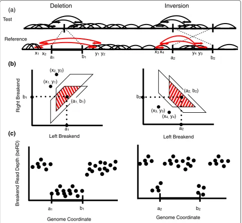
Although researchers typically focus on common classes of SVs, such as deletions and inversions, more generally a SV corresponds to a rearrangement creating one or more novel adjacencies between pairs of loca-tions in the reference genome. That is, two localoca-tionsa andb, which were originally separated in the reference genome, are now adjacent in the test genome. For example, a deletion creates one novel adjacency while an inversion creates two (Figure 1a). Following the ter-minology of VCF (Variant Call Format) version 4.1 [45], we refer to locations aandb individually as breakends and as mated breakends when paired at either end of a SV created by a rearrangement.

We define a predicted SV V as a pair V = (F,B) where F={f1,f2,. . .,fk} is a set of k discordant

frag-ments containing the novel adjacency, and B is the breakend polygon, a region describing all possible mated breakends (a,b) determined by the discordant fragment mappings (Figure 1b). The breakend polygon is defined by the positions of the mapped ends of each fragment and the minimum (Lmin) and maximum (Lmin) length of fragments. If V is a true SV, then there is an ordered pair (a,b)∈B corresponding to a novel adjacency cre-ated by the rearrangement. That is, there is a (a,b)∈B such thata and b are the breakends of the SV in the reference genome. (See Materials and methods and [33] for more information on how the breakend polygon is defined.)

Discordant and concordant fragments provide comple-mentary information about a variant. Discordant frag-ments define the breakend polygon B while concordant fragments (or lack thereof) provide additional informa-tion about the precise locainforma-tion of the breakends within the polygon. Ifaandb represent mated breakends cre-ated by a deletion, inversion or other rearrangement in the reference genome, we should see a decrease in the coverage by concordant fragments at these points. The type of signal we expect to see depends on the type of SV present (Figure 1c). For a deletion, we expect a drop in the coverage of concordant fragments throughout the genomic interval [a,b]. This is commonly known as the RD signal and has previously been exploited to reveal copy number variants [38]. For an inversion or reciprocal translocation, we expect a sharp drop in coverage in the regions immediately surroundingaandbas many of the fragments containingaorbin the test genome are dis-cordant when mapped to the reference. However, there is

no drop in coverage‘inside’the inversion or transloca-tion. We define this highly local drop in coverage as the breakend read depth (beRD) signal.

We develop a probabilistic model based upon the mapped locations of all fragments, concordant and dis-cordant, in the test genome. By doing so we integrate both the presence of discordant fragments (PR signal) and concordant coverage (RD signal) into a single prob-abilistic method, GASVPro. In addition, GASVPro directly estimates the location of the breakends aandb for a SV V and classifies the prediction as homozygous or heterozygous. We first present our model in the restricted context where every fragment has a unique mapping to the reference genome. Then, we extend our model to fragments with multiple alignments by using an MCMC approach to sample over the possible map-pings for each fragment.

Probability of a structural variant

We determine the probability of a potential SV V by considering the number,k, of discordant fragments as well as the beRD, the depth of coverage at each candi-date breakend. By doing so, we directly estimate the novel adjacency created by V by considering all possible mated breakends consistent with the discordant frag-ments. Since our formulation depends only on the pro-cess of sampling fragments from the test genome, and not on the class of variant, our probabilistic model is applicable to generic rearrangements.

We follow the Langer-Waterman model [46] of sequencing and assume that the starting positions of the fragments are sampled from the test genome uniformly so that the left positions of fragments follow a Poisson process with parameter l. If all sequenced fragments had fixed lengthL, the number of fragments containing an arbitrary point pfrom the test genome, called the coverage ofp, would simply be the number of fragments sampled with left endpoint in the interval [p-L+ 1,p]. According to the Poisson process, the coverage of a point pfollows a Poisson distribution with meanlL. In general, we do not know the size of any particular frag-ment and thus we use the average fragfrag-ment length, Lavg,

and model the coverage ofpby a Poisson distribution with mean λc=λLavg.

Ifpis sufficiently far from all sites of structural varia-tion, we expect all sequenced fragments containing pto be concordant with respect to the reference genome. However, ifpis the breakend of an SV, coverage will be reduced, as there will be fewer concordant fragments containing the breakend. In particular, the distribution of the number of fragments containing a breakendpis approximated by a Poisson distribution with mean λd= (Lavg−2×readlength)λ (see Materials and

Consider a candidate SV V = (F,B). If V is a true SV, then there is an ordered pair, (a,b)∈B, corresponding to a novel adjacency in the test genome created by the rearrangement. As such, the number of concordant frag-ments containing aorb should be lower than expected for an arbitrary point in the reference genome. Alterna-tively, if V is not a true SV, then the coverage of points aandb by concordant fragments will follow the Poisson distribution with mean λc. We next describe the

prob-ability of a variant V by conditioning on the choice of breakends and number of copies of the novel adjacency (a,b) in the test genome. Specifically, for a candidate novel adjacency (a,b)∈B, letC(a,b) = {0,1,2} indicate the number of copies of the novel adjacency in the test genome. (Here we are considering only copy-neutral or copy number loss events (for example, deletions) and not duplications. The extension to the latter case is future work.) We consider three events: (1)aandb are breakends of a homozygous SV, (C(a,b) = 2); (2) aand b are breakends of a heterozygous SV (C(a,b) = 1); (3)a andb are not SV breakends (C(a,b) = 0).

For a candidate breakend p, we define the breakend read depth (beRD),n(p), to be the number of mapped fragments containingp. In the case thataandbare end-points of a homozygous SV, we expectn(a) =n(b) = 0; that is, any concordant fragment containingaorb repre-sents a mapping error. We assume that mapping errors are independent and the probability, perr, of an erroneous

mapping is the same for all fragments. In addition, the number,k, of discordant fragments in F is drawn from a Poisson distribution with parameter λd. Thus,

condi-tional on a choice of breakends (a,b), the probability that V represents a homozygous SV (that is, C(a,b) = 2) is given by:

P(V|C(a,b) = 2) =

pnerr(a)+n(b)

Pois(λd;k) (1)

where Pois(λ;k) =λkexp(−λ)/k! is the probability density function for the Poisson distribution with mean l. One could explicitly define the unconditional prob-ability that V is a homozygous variant by examining the likelihood that each pair (a,b)∈Bare the true mated breakends. Instead, we make a simplification by taking the maximum probability over all possible breakend pairs:

P(V|C(B) = 2) = max

(a,b)∈BP(V|C(a,b) = 2) (2)

where byC(B) = 2 we mean the breakpoint region B defines a homozygous SV.

Similarly, if (a,b)∈B are mated breakends of a het-erozygous variant,C(a,b) = 1, we expect the number of

concordant fragments that contain a or b to follow a Poisson distribution with mean λc/2and the number of

discordant fragments that contain the novel adjacency (a,b) to follow a Poisson distribution with mean λc/2,

respectively. Thus, conditional on the choice of break-ends (a,b), the probability that Vrepresents a heterozy-gous SV is given by:

P(V|C(a,b) = 1) =Pois

λc 2;n(a)

Pois

λc 2;n(b)

Pois

λd 2;k

(3)

As before, we define the unconditional probability that V represents a heterozygous variant by:

P(V|C(B) = 1) = max

(a,b)∈BP(V|C(a,b) = 1) (4)

Finally, if aandb, (a,b)∈B, are not breakends of a SV, C(a,b) = 0, we expect the number of concordant fragments containing the breakpoints n(a) and n(b) to follow Poisson distributions with meanlc and allk dis-cordant fragments to be mapping errors, each occurring independently with probability perr. Thus, conditional

on a choice of (a,b), the probability that V does not represent a SV is given by:

P(V|C(a,b) = 0) =Poisλc;n(a)

Poisλc;n(b)

perrk(5)

As before, we define the unconditional probability that V is not a variant by:

P(V|C(B) = 0) = max

(a,b)∈BP(V|C(a,b) = 0) (6)

For each candidate variant we decide between alterna-tives using a likelihood ratio. That is, we compare the probability that V represents a SV (homozygous or heterozygous) with the probability that V is an error as follows:

(V) = max

(a,b)∈B

max{P(V|C(a,b) = 2),P(V|C(a,b) = 1)}

P(V|C(a,b)) = 0 (7)

In practice we report variants V where log(V) exceeds a prescribed threshold. In addition to assigning a likelihood to a SV, our formulation determines a max-imum likelihood estimate for the novel adjacency (a,b) and if a variant is homozygous or heterozygous.

Probability of a deletion

fragments and define amax= arg max

a {

(a,b)∈B} _and

bmin= arg min b

{(a,b)∈B}_{. Then, for any choice of}

mated breakends (a,b)∈B, the interval I(B) = [amax,bmin] must be deleted. As before, we

expect the numbern(I) of concordant fragments whose mappings overlap the interval I(B) to be Poisson dis-tributed with mean:

λI =λ

(bmin−amax)+Lavg

Let C(B) = {0,1,2} be the number of copies of the var-iant in the test genome. We consider the probability of three events:

PV|C(B) = 2=

pnerr(I)

Pois(λd;k) PV|C(B) = 1=PoisλI/2;n(I)

Poisλd/2;k

PV|C(B) = 0=PoisλI;n(I) pkerr

and finally the likelihood of a deletion compared to a mapping error:

(V) = max

PV|C(B) = 2,PV|C(B) = 1

PV|C(B) = 0 (8)

There are several additional factors we consider when using our model on sequencing data. First, there are fac-tors other than SVs that can impact the coverage of con-cordant fragments over an interval. As such, to adjust for differences in the ability to map reads throughout the genome, in our model for deletions we scale the number of concordant fragments by the local mapability of the putative deleted interval. Second, since in this study we are primarily interested in inversion and deletion SVs, in practice we utilize a heuristic to eliminate regions of the genome with extremely high coverage by concordant fragments. Further information on these practical details are given in the Materials and methods section.

Selecting a mapping for each fragment

In the previous sections, we assumed that there was a single high-quality alignment for all reads and therefore one high-quality alignment for each fragment. However, some reads may have multiple high-quality alignments due to repetitive sequences in the reference or sequen-cing errors in the reads. Selecting one of the possible alignments for each read from the pair defines an align-ment of the fragalign-ment. Since each fragalign-ment represents a unique contiguous region of the test genome, at most one alignment is the correct one and we refer to this as the mapping of the fragment.

Selecting a mapping for each fragment defines the set of concordant and discordant fragments and an asso-ciated set of SVs that could be evaluated using the model

in the previous section. Although any such selection defines a fragment configuration consistent with the data, each selection has a different probability. Thus, rather than selecting a mapping for each fragment in advance, we consider the space of all possible mappings for all fragments and use a MCMC approach to sample from the space of possible mappings in proportion to their probability.

With these distinctions, we now revisit our notions of ‘concordant’ and‘discordant’from above. A concordant fragment is a fragment whose unique mapping is con-cordant. That is, both reads have a single high-quality alignment to the reference and the alignments are con-cordant with respect to the sequencing process. A dis-cordant fragment is a fragment whose entire set of alignments are discordant. (Note, this formulation ignores any fragment with multiple alignments, at least one of which is concordant.)

Let F=f1,f2,. . .,fm be the set of all discordant

fragments. Suppose that the two reads from a fragment f ∈F map tos andt locations, respectively. An ment of a fragment corresponds to selecting an align-ment for each read, and thus we define A(f) ={(xi,yj)}

where i = 1,2,...s and j = 1,2,...t as the set of all align-ments for a fragment f, only one of which may be the true mapping. Let A=A(f1

,A(f2),. . .,A(fm) be the

set of alignments for all fragments.

Let V={V1,V2,. . .,Vn} be a set of candidate SVs

supported by _A, as before Vi=(Fi,Bi). V is computed

by clustering discordant pairs that support the same var-iant. (In the results below, we use GASV [33] to obtain the breakpoint polygon associated with each Vi;

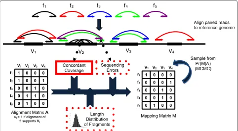
how-ever, this step could be replaced by a different clustering method.) We represent the set of all possible SVs sup-ported by _A with anm×nbinary (0-1 valued)alignment matrix, A= [aij], with rows corresponding to fragments

f1,f2,. . .,fm and columns corresponding to possible

SVs {V1,V2,. . .,Vn}. Here aij= 1 if fragment fi

sup-ports SV Vj (that is, there is an element of A(fi) that

supports variant Vj and thus fi∈Fj) and aij= 0

other-wise (Figure 2).

We assume that a discordant fragment supports at most one SV. Thus, our goal is to select the single ‘ cor-rect’mapping for each fragment, according to some cri-terion. Such a selection corresponds to a binary m×n mapping matrix M=mij

, where mij= 1 if fragment fi

is assigned to SV Vj. M satisfies the following:

1. mij≤aij; that is, mij= 1 only if aij= 1,

2.

i

mij≤1_{for all i; that is, each row in M has at}

Finally, as before, the probability of variants depends on the associated copy number, C(B), of a variant. We explicitly distinguish between homozygous and hetero-zygous SVs by including a binary vector C=(C1,C2,. . .,Cn) where Cj=C(Bj). If any

discor-dant fragments are assigned to Vj, we require Cj>0.

Together C and M define the differences between the test and reference genome.

Probability of a mapping matrix

Our dataDconsists of a set_F of discordant fragments, a set _A of alignments, a set _V of possible SVs, and the positions of all concordant mappings in the genome. We next generalize our probability model from the previous section to the probability of a mapping matrix based on the generation of the dataDfrom a given genome.

For a mapping matrix M and discordant fragment fi,

let γi(M) denote the column index of the 1 in the i-th

row, or 0 if fi is not assigned. For a mapping matrix M

and a variant Vj, let Rj(M)be the set of rows with a 1

in columnj. The support, Sj(M), of variantjis defined

as the number of assigned discordant fragments:

Sj(M) = Rj(M)=

i mij

Finally, we define the total number of variants V(M) predicted by M:

V(M) = {j:Sj(M)>0}.

Given an alignment matrix A, the probability of a mapping matrix M is a function of the number of frag-ments supporting each variant with positive support. We assume that the number of variants with positive support follows an exponential distribution with para-meter η >0. Finally, if a discordant fragment is assigned to none of the SVs, then this fragment repre-sents a mapping error, an event with probability perr.

Thus, we have:

P(M,C|A)∝ηe−ηV(M)

j:Sj(M)>0

P(Vj(M)|Cj(M))

i:γi(M)=0 perr₍₉₎

where Vj(M) = (Fj(M),Bj(M)) is the SV in column j

supported by fragments Fj(M), corresponding

Mapping Matrix M

Alignment Matrix A

aij = 1 if alignment of fi supports Vj

Align paired reads to reference genome

Concordant Coverage

Sequencing Errors

V

V

V

Sample from

Pr(M|A)

(MCMC)

Length Distribution of Fragments

X

V

1 0 0 0 1 0 0 1 0 0 1 0 0 1 1 0 0 1 0 0 V1 V2 V3

f1

f2

f3

f4

V4

f

f

f

f

f

f5

1 0 0 0 0 0 0 1

0 0 1 0 0 0 1 0 0 1 0 0 V1 V2 V3 f1

f2

f3

f4

V4

f5

breakpoint region Bj(M) and Cj(M) =C(Bj(M)). As

above, we utilize a different model for predicting dele-tions that also includes read depth inside the putative deleted interval. Finally, we define P(M|A) by defining C by selecting the most likely copy number Cj for

eachj:

P(M|A) = max

C P(M,C|A). (10)

Note that M specifies a unique mapping for each frag-ment supporting a variant; thus, one solution would be to consider P(M|A) over all possible mapping matrices. However, because the number of possible mapping matrices M grows exponentially with the number of frag-ments, we use a MCMC procedure to efficiently sample from the space possible mapping matrices M (Figure 2; Section A2 and Figures A2, A3 in Additional file 1). Our MCMC procedure converges to the unique stationary dis-tribution given in Equation 10.

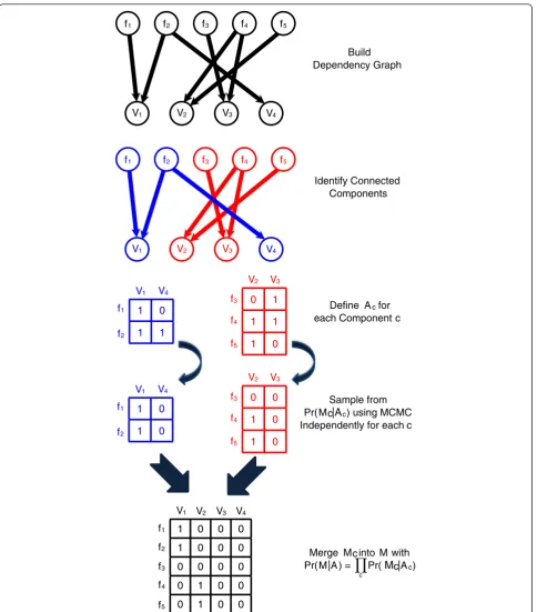
Although the space of mapping matrices has high dimension, our MCMC procedure remains computation-ally tractable because our sampling procedure may be performed on disjoint sets of fragment mappings and the variants they support. Thus, our MCMC samples inde-pendently on each such component and the combination of these samples converges to the same stationary distri-bution as sampling over the complete space. See Figure 3 for a schematic. In the Materials and methods section, we provide a complete description of our MCMC sampling procedure and provide further discussion in Additional file 1.

Deriving the predicted structural variants

Our MCMC procedure samples mapping matrices in proportion to their probability P(M|A); however, our ultimate goal is to report a final set of SV predictions. One approach to SV prediction is to select a single M according to some criteria; for example, the M that minimizes the total number of SVs predicted. This approach is used by a number of SV detection methods that consider multiple assignments for fragments, such as VariationHunter [42] and Hydra [34]. We instead predict SVs by considering the entire space of mapping matrices M according to P(M|A) as described in the Materials and methods. In practice, we found only minor differences in the receiver operating characteristic (ROC) curves for the different reporting methods we considered (Figure A4 in Additional file 1).

Results on sequenced data

We applied GASVPro to simulated paired-end data on the Venter Genome (HuRef) [47], as well as two pre-viously sequenced human genomes, NA18507 [14] and a European individual, NA12878, from the 1000 Genomes

study [44]. We also compared results from GASVPro to two previously published methods, Hydra [34] and BreakDancer [32], as well as the original GASV. (We also performed some comparisons with VariationHunter [42]. Since results were strikingly similar to Hydra, as previously noted in [34], and we were unable to process the full datasets for NA12878 and NA18507 using the current publicly available distribution of VariantionHun-ter, we present only the results for Hydra.) Finally, we compare to CNVer, a method combining RD and PR to detect copy number variants [38].

These methods, and other similar SV prediction pro-grams, typically employ several steps, including align-ment of reads to the reference genome, predicting SVs from alignments, post-processing predictions (for exam-ple, pruning a set of predicted SVs to remove redun-dancy) and comparison to known variants. In an effort to directly compare the performance of the SV predic-tion algorithms, rather than the specific pre- and processing steps, we standardized the alignment, post-processing and comparison steps. In particular, we used the same read alignments for all methods. (Note this involved modifying the source code for Breakdancer to consider only a user-specified set of discordant frag-ments.) For GASVPro and Hydra, the methods that allow fragments to have multiple possible alignments, we realigned reads to the reference genome with Novoa-lign [48] and distinguish results on the full set of aNovoa-lign- align-ments (GASVPro and Hydra) from results on only the high-quality unique alignments (GASVPro-HQ or Hydra-HQ). Before comparing results, redundant pre-dictions were removed with the same pruning procedure for each method (see Materials and methods).

Simulated data

We first test GASVPro on simulated data generated from the Venter genome [47]. We produced a synthetic

dataset by inserting the list of annotated SVs on chro-mosome 17 of Venter’s genome (8,801 deletions, 8,572 insertions and 4 inversions) into the human reference

f1 f2 f3 f4 f5

V3

V1 V2 V4

1 0

1 1

V1 V4

f1

f2

0 1

1 1

1 0 V2 V3

f3

f4

f5

Sample from Pr(Mc|Ac) using MCMC Independently for each c

Identify Connected Components

0 0

1 0

1 0 V2 V3

f3

f4

f5

Define Ac for each Component c

1 0

1 0

V1 V4

f1

f2

1 0 0 0

1 0 0 0

0 0 0 0

0 1 0 0

0 1 0 0

V1 V2 V3 f1

f2 f3 f4

V4

f5

f1 f2 f3 f4 f5

V3

V1 V2 V4

Build Dependency Graph

Merge Mc into M with Pr(M|A) = Pr(Mc|Ac)

c

genome (hg18). These SVs varied in length from one to several thousands of bases. We simulated 100× coverage of this chromosome by 50-bp PRs with a mean fragment length of 200 bp and a standard deviation of 20 bp using the SAMtools wgsim program [49]. For all meth-ods, the resulting sets of predictions were pruned and compared to known variants with the double uncer-tainty metric with reference unceruncer-tainty set to 0 (see Materials and methods).

The lengths of deletions that are readily predicted from PRs depend on fragment size [11]. To mirror the procedures used on the sequenced genomes, we only considered fragments with mapped length ≥2×Lmax (where Lmax= 293) as potential deletions. We compared predictions from all methods to the 124 deletions with length ≥125 bp. Figure 4 compares all methods on this data set; compared with GASV, Breakdancer and Hydra, GASVPro is over 50% more specific at maximum sensitivity.

All methods had greater sensitivity than CNVer, which made 218 predictions but detected only 3 deletions with the double uncertainty metric. The lower sensitivity of CNVer can be explained in part by internal filtering: the published code of CNVer reports only copy-number events that are larger then 1 kb, which eliminates all but 9 out of 124 simulated deletions. In addition, the reported coordinates from CNVer lie farther from true breakends, although the predicted deletion interval

typically contains the true deletion. We note that 16 of 218 CNVer predictions completely contained a true deletion, including 5 of 9 deletions larger than 1 kb. Thus, some of the difficulties with CNVer result from how it merges potential copy-number variants before reporting a final set of predictions (Section A3 in Addi-tional file 1).

We next discuss GASV compared with Breakdancer, Hydra and Hydra-HQ. Before removing redundant pre-dictions by pruning, GASV predicts 648 deletions with at least one supporting fragment, which detects 60 Ven-ter deletions. Thus, the maximum sensitivity is 48%. A common method to increase specificity is to increase the minimum number of supporting fragments for a prediction. As discussed previously, however, many pre-dictions from SV methods overlap. Removing these overlapping predictions (see Materials and methods) improves performance more than increasing the number of supporting fragments. For GASV, restricting the set of predictions to those with at least two supporting frag-ments results in 244 predictions but detects only 46 deletions. In comparison, pruning the 648 predicted deletions with at least one fragment retains 347 predic-tions that detect 57 true delepredic-tions. In comparison, Hydra-HQ and Hydra had slightly lower sensitivity, pre-dicting only 44 deletions at maximum sensitivity, but had similar overall performance to GASV. Breakdancer had similar performance throughout with slightly higher

0 10 20 30 40 50

0 10 20 30 40 50 60

T

rue

P

os

iti

ves

False Positives

Simulated Venter Deletions

Hydra GASVPro High/Low Quality and Ambiguous Alignments

GASVPro-HQ

Hydra-HQ GASV Breakdancer High Quality Alignments

CNVer

sensitivity than Hydra/Hydra-HQ and GASV and equal specificity.

The integrative probabilistic model used by GASVPro greatly improves specificity. Analyzing only high quality unique mappings, GASVPro-HQ predicts only 64 dele-tions with positive log likelihood, log(V)> 0, which include 50 true deletions. Note that these 64 predictions are a subset of those predicted by GASV. Thus, com-pared to GASV, GASVPro-HQ has a substantially lower false positive rate at highest sensitivity. The improved specificity of GASVPro-HQ over GASV is evidence that our likelihood statistic is a better predictor of true var-iants than the number of supporting fragments (see also Figure A7 in Additional file 1 for a comparison). Includ-ing low-quality and ambiguous alignments increases the space of possible variants substantially without signifi-cantly increasing the number of detectable deletions. That is, the full set of possible alignments suggest 1,051 potential deletion events that overlap, at most, 61 out of 124 true deletions. However, GASVPro has similar per-formance to GASVPro-HQ throughout. This suggests that the MCMC sampling method is able to successfully eliminate many false positive predictions even with a much larger number of initially possible variants.

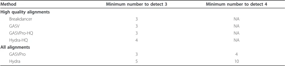
Finally, we compared the ability of all methods to identify the four inversions on Venter chromosome 17 (Table 1). On this simulated data our probabilistic for-mulation and MCMC sampling method proved benefi-cial. GASVPro-HQ identified three inversions with four predictions while GASVPro identified all four inversions with no false positive predictions. Notably, the addi-tional inversion identified by GASVPro had breakends within a segmental duplication. In this case a total of 170 fragments had two possible alignments, each of which corresponded to a potential inversion SV, but only one of which is the true inversion. The beRD signal used by GASVPro allowed the algorithm to successfully distinguish between the true and false prediction. The MCMC algorithm used by GASVPro assigned a greater likelihood to the true prediction because 23 concordant

fragments map to the breakend polygon for the false prediction. In comparison, Hydra requires ten predic-tions to detect all four inversions. GASV and Breakdan-cer are slightly less sensitive, detecting only three quarters of known inversions. Thus, GASVPro is the only method to attain optimal sensitivity and specificity on the inversion data set.

Sequencing data

NA12878 deletionsWe next compared the methods on Illumina sequencing data of a CEU individual, NA12878, from the 1000 Genomes Project. There are two sets of validated SVs available for this individual. First, deletions and inversions were validated from a previously published fosmid study [16] and deletions were separately validated as part of the 1000 Genomes Project [44]. In addition, the validated deletions from the 1000 Genomes data set were also annotated as homozygous or heterozygous.

Individual NA12878 was sequenced in both Pilot 1 (≈4× coverage) and Pilot 2 (≈40× coverage) of the 1000 Genomes Project. For Pilot 1, a single library was sequenced with a read length of 37 bp and an average fragment size of 230 bp. For Pilot 2, multiple libraries were sequenced with read lengths from 37 to 52 bp and an average fragment size of 150 to 350 bp. Thus, we analyzed both datasets to examine the effect of different coverage on the ability of methods to predict SVs.

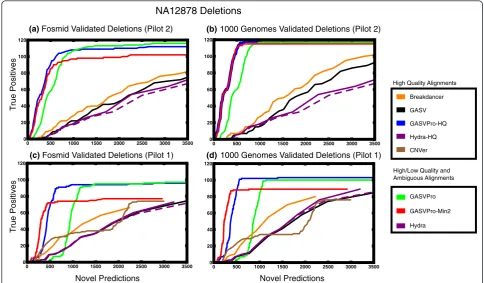
In Figure 5 we plot‘ROC curves’comparing the pre-dictions of GASV, GASVPro, GASVPro-HQ, Hydra, Hydra-HQ, CNVer and Breakdancer on data from Pilot 2 (Figure 5a,b) and Pilot 1 (Figure 5c,d) to both sets of validated deletions. Since CNVer could only be run on a single library, we consider CNVer results on Pilot 1 data alone. Because the complete list of true SVs in the gen-ome is not yet known, we cannot compute the number of false positives/negatives. Thus, we plot the number of novel predictions compared to true positives. We also considered only predictions with at least two supporting fragments and plot these results as GASVPro-Min2. As before, to assess the difference due to low quality and

Table 1 Comparison of performance of methods with respect to identifying the four inversions on Venter chromosome 17

Method Minimum number to detect 3 Minimum number to detect 4

High quality alignments

Breakdancer 3 NA

GASV 3 NA

GASVPro-HQ 3 NA

Hydra-HQ 4 NA

All alignments

GASVPro 3 4

Hydra 5 10

ambiguous mappings, we plot both Hydra and Hydra-HQ; the latter is Hydra run on only high-quality uniquely mapped fragments.

We first consider the results on the higher coverage Pilot 2 data (Figure 5a,b). Four curves represent methods run on only uniquely mapped fragments: GASV, GASV-Pro-HQ, Hydra-HQ and Breakdancer. Breakdancer has slightly improved performance compared to Hydra-HQ and GASV, attaining equal sensitivity with up to 200 fewer predictions throughout. However, this may be an artifact of Breakdancer’s aggressive clustering procedure (discussed in Section A3 of Additional file 1). GASVPro-HQ has the best overall performance with over a 85% reduction in novel predictions at highest sensitivity com-pared to Breakdancer, GASV and Hydra.

Of the three methods that use all alignments (GASVPro, GASVPro-Min2 and Hydra), GASVPro has the highest sensitivity, detecting 119 of 139 true deletions with 19,715 novel predictions on the set of validated deletions from the 1000 Genomes study. By increasing the minimum like-lihood threshold, and thus reducing the number of predic-tions, GASVPro predicts 114 of 139 true deletions with only 907 novel predictions; this represents a 95% decrease in the number of novel predictions with only a 3% decrease in true positives. GASVPro-Min2 has higher

specificity than GASVPro, making around 200 fewer pre-dictions than GASVPro at equal sensitivity. Notice the addition of ambiguous mappings alone does not greatly improve performance as the behavior of Hydra and Hydra-HQ is very similar, with Hydra being slightly more sensitive. Thus, regardless of whether unique or ambigu-ous fragments are used, combining both read depth and PRs with our probabilistic model (GASVPro-HQ, GASV-Pro-Min2 or GASVPro) results in significant improve-ments to sensitivity and specificity.

In addition to improving the ability to successfully pre-dict true deletions, our probabilistic model also accu-rately classifies these variants as homozygous or heterozygous. GASVPro-HQ correctly classified 104 out of the 119 known deletions with highest likelihood as homozygous or heterozygous according to the annota-tions in the 1000 Genomes data set. Remarkably, all 28 homozygous variants in this set were correctly classi-fied even though some had fewer supporting discordant fragments than many correctly classified heterozygous variants.

On Pilot 1 data, we also compare the performance of CNVer, which uses both discordant mappings and read depth to predict copy number variants. In contrast to the simulated data set above, all known deletions analyzed

(c) Fosmid Validated Deletions (Pilot 1) (d) 1000 Genomes Validated Deletions (Pilot 1)

T

rue Positives

NA12878 Deletions

(a) Fosmid Validated Deletions (Pilot 2) (b) 1000 Genomes Validated Deletions (Pilot 2)

T

rue Positives

Novel Predictions Novel Predictions

Hydra GASVPro-Min2 GASVPro High/Low Quality and Ambiguous Alignments

GASVPro-HQ

Hydra-HQ GASV Breakdancer High Quality Alignments

CNVer

0 500 1000 1500 2000 2500 3000 3500

0 20 40 60 80 100 120

0 500 1000 1500 2000 2500 3000 3500

0 20 40 60 80 100 120

0 500 1000 1500 2000 2500 3000 3500

0 20 40 60 80 100 120

0 500 1000 1500 2000 2500 3000 3500

0 20 40 60 80 100 120

here are larger than 1 kb and thus CNVer attains similar sensitivity to PR methods, like Hydra, GASV and Break-dancer. However, the number of discordant fragments per prediction, the criteria used to rank results for PR methods, provides a better trade off between true and false positive predictions than the estimated depth of coverage, which we use to rank CNVer predictions.

Even with the reduced coverage, compared to Pilot 2, the benefits of our probabilistic models are evident, and GASVPro outperforms all competing methods. GASV-Pro-HQ and GASVPro-Min2 have improved perfor-mance compared to Hydra, Hydra-HQ, Breakdancer and GASV. Note that the specificity for GASVPro drops below all other methods at the highest likelihood thresh-old (Figure 5c,d). This drop in performance is due to many predictions of GASVPro consisting of only a single discordant fragment mapping to a large region with very few concordant fragments. While it is possible these are true variants, it is more likely that most of them are false positives and, as such, eliminating these predictions (GASVPro-Min2) restores performance to that obtained by GASVPro-HQ. On this dataset, GASVPro-HQ cor-rectly classifies 84 out of the 102 known deletions with highest likelihood as homozygous or heterozygous. As in the Pilot 2 data set, all 26 of 102 homozygous deletions were correctly classified, 3 of which have fewer than 3 supporting fragments.

We next evaluate the effect of increased coverage on each method by comparing the results from Pilot 2 (Figure 5a,b) with Pilot 1 (Figure 5c,d). For the methods utilizing only discordant mappings (Hydra, Hydra-HQ, GASV, and Breakdancer) performance is similar between Pilot 1 and Pilot 2 data. In contrast, performance of our probabilistic methods, GASVPro-HQ, GASVPro-Min2 and GASVPro, increases substantially with coverage. The maximum sensitivity of GASV Pro and GASVPro-HQ increases by about 20% on both data sets, from 97 to 119 and 96 to 114, respectively, for the fosmid validated set and 100 to 119 and 103 to 120 on the 1000 Genomes validated set. This improved performance results from integration of both discordant fragments (PR signal) and concordant fragments (RD signal). Increasing the sequen-cing coverage increases both discordant and concordant mappings throughout the genome. However, higher dis-cordant coverage contributes to both true and false pre-dictions, and thus methods that analyze only discordant fragments are less able to leverage the increased coverage to distinguish true from false predictions. In contrast, increased coverage by concordant fragments leads to sharper delineations between normal and deleted regions in the genome. Although it is possible that CNVer results would have also improved with the higher coverage data, a comparison was not possible as multiple libraries are not supported in the published CNVer implementation.

Finally, we remark on a practical difficulty in assessing the performance of methods on sequenced genomes. As indicated above, the complete set of SVs on these gen-omes is unknown. Thus, it is possible that predictions classified as‘novel predictions’could in fact be true, but yet unknown, variants. In addition, the set of validated variants that we use as true positives may not be repre-sentative of all SVs in these genomes. For example, we attained significant improvements in specificity for both inversions and deletions on NA12878 when we used a ‘homozygous-only” model in GASVPro (Figure A8 in Additional file 1). This suggests that the set of known variants may underrepresent heterozygous deletions and inversions, which are presumably more difficult to detect and validate.

NA18507 deletions We next compare all methods on previously published Illumina data [14] for the YRI indi-vidual NA18507. This genome was sequenced to high coverage (35 bp reads, ≈200 bp fragment length, 30× coverage) and, as for NA12878, there were two available validated sets of deletions and one set of inversions. In Figure 6, we show the results for previously validated fosmid deletions (Figure 6a) and validated deletions from the 1000 Genomes Project (Figure 6b). Since CNVer published their predictions on this data set, we compare directly to their previously reported results.

As above, employing our integrative probabilistic model for discordant fragments with unique mappings, GASVPro-HQ greatly improves performance compared to the original GASV. Using GASV alone, at maximum sensitivity we predict 55 of 93 deletions from the fosmid study with 2,240 novel predictions. In comparison, GASVPro-HQ successfully predicts the same 55 of 93 deletions with only 573 novel predictions. Similarly, for the 1000 Genomes deletions, at maximum sensitivity GASV predicts 95 of 118 deletions with 2,201 novel pre-dictions while GASVPro-HQ attains the same sensitivity with only 1,372 novel predictions. Thus, using our prob-abilistic framework provides a two-fold increase in speci-ficity at equal sensitivity. On the fosmid validated deletions, CNVer attains higher sensitivity than other methods and has overall higher specificity than GASV or Hydra at equal sensitivity (Figure 6a). However, this per-formance is not maintained on both sets of validated deletions (Figure 6b).

Although both GASVPro and original GASV match 70 of 93 variants from the fosmid study and 95 of 118 from 1000 Genomes Project, this is at the expense of predict-ing thousands of novel deletions on each data set, 5,535 and 21,523, respectively. We attain improved perfor-mance on the ambiguous data set by considering predic-tions with more than one supporting fragment, GASVPro-Min2; however, these results are still worse than GASV alone.

The decreased performance of GASVPro and Hydra on this data set, compared to NA12878 above, cannot be solely attributed to the read length as in both cases the sequenced reads were, on average, the same length,

37 bp. The differences seem likely due to difficulties in mapping uniquely to the reference. For NA12878, 31% of all mappings were unique while for NA18507, less than 1.5% of mappings were. In addition, there were more dis-cordant fragments considered for NA18507, but fewer validated SVs. This combination may explain the sub-stantial increase in‘novel’predictions, as compared to known deletions.

InversionsIn comparison to deletions, inversion SVs are more difficult to analyze for three reasons. First, there is no difference in read depth across the inversion, but only a change in read depth at the break ends (break end read depth). Second, there are few known inversion

NA18507 Fosmid Validated Deletions

Novel Predictions

True Positives

True Positives

NA18507 1000 Genomes Validated Deletions

(a)

(b)

Hydra

GASVPro-Min2 GASVPro High/Low Quality and Ambiguous Alignments

GASVPro-HQ

Hydra-HQ GASV Breakdancer High Quality Alignments

CNVer

0 500 1000 1500 2000 2500

0 20 40 60 80

0 500 1000 1500 2000 2500

0 20 40 60 80 100

variants available for testing. Indeed, the 1000 Genomes SV paper [43] reports thousands of deletions but no inversions. Third, inversion SVs are known to have breakpoints with segmental duplications or other repeti-tive sequences, and aligning reads to these regions is complicated.

Even with these limitations we demonstrate the bene-fit of beRD in improving inversion prediction. As noted previously, on the simulated data set the beRD signal allowed GASVPro to correctly assign fragments to the true prediction when there were two choices possible. We now illustrate the beRD signal is beneficial on the real data. In Figure 7, we show the beRD for two inver-sions identified in NA18507 by GASVPro-HQ. As expected, in both cases there is a noticeable drop in coverage near the potential breakends, demonstrating the benefit of a model that utilizes beRD in addition to discordant fragments.

We compared predicted inversions for all methods to a set of validated inversions from a previous fosmid study [16] (see Materials and methods). The number of vali-dated inversions is significantly smaller than the number of validated deletions; 23 inversions were validated in NA12878 and 10 in NA18507. All methods were far less sensitive in identifying inversions than deletions; maxi-mum sensitivity over all methods was less than 20% on NA12878 and 70% on NA18507.

For all methods, we show the minimum number of inversion predictions needed to identify 1, 2 and 3 out of 23 inversions for NA12878 Pilot 1 and Pilot 2 data (Table 2). On Pilot 1 data our probabilistic models GASVPro and GASVPro-HQ attained improved sensitiv-ity compared to GASV when detecting one and two

inversions. In the case of the first inversion, the specifi-city increased by over 50% for GASVPro and over 80% for GASVPro-HQ. In almost all cases the higher coverage from Pilot 2 improved performance as the same number of inversions are detectable with fewer predictions. How-ever, unlike for deletions, our probabilistic models do not always attain highest specificity. Over all methods, GASV was able to detect 2 inversions with the minimum num-ber of predictions, while GASVPro-HQ detected 1 and 3 inversions with the minimum number of predictions. Finally, including lower quality mappings on this dataset did not yield improved performance; although GASVPro was able to attain highest sensitivity, detecting 4 of 23 inversions, this came at the price of thousands of more predictions.

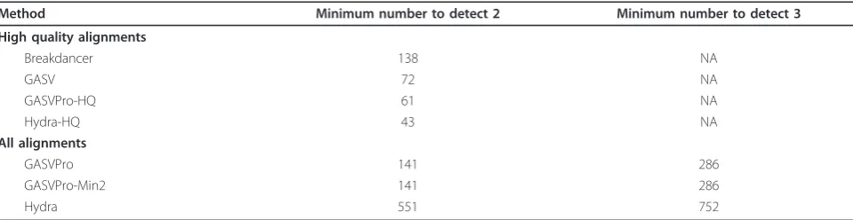
Lastly, we analyze inversion results for NA18507 (Table 3). A total of two out of ten inversions are pre-dicted from unique discordant mappings alone. All methods are able to predict these inversions, but Hydra-HQ is able to do so with only 43 predictions, the mini-mum number across all methods. As in the simulated Venter data, a third true inversion is detected with the inclusion of ambiguous mappings. In this case, GASV-Pro and GASVGASV-Pro-Min2 detect three of ten inversions with 60% fewer predictions than Hydra. Thus, while the probabilistic model used by GASVPro is beneficial in some cases, unlike for deletion variants, it does not result in improved specificity for all cases.

Discussion

We introduce GASVPro, a method for SV detection that: (1) integrates both the RD signal (including the more localized beRD) and PR signal of structural variation into

8.9060 107 8.9065 107 8.9070 107 8.9075 107 8.9080 107 8.9085 107 0

50 100 150

1.07272 108 1.07274 108 1.07276 108 1.07278 108 1.07280 108 1.07282 108 0

50 100 150

Position

Position

C

overage

(b)

(a)

a single probabilistic model; (2) analyzes multiple possi-ble read alignments using an MCMC procedure; and (3) explicitly defines uncertainty in the breakends of a var-iant. GASVPro is the first method to utilize a probabilis-tic formulation to identify generic SVs and not only copy number variants. We demonstrated that, compared to the previously published methods Breakdancer, Hydra and GASV, GASVPro has significantly higher specificity at equal or greater sensitivity in detecting known var-iants. Finally, our method is easily generalized to include additional signals predictive of variants.

The increased specificity and sensitivity of GASVPro demonstrates the benefit of integrating multiple signals of structural variation into a probabilistic model. In particu-lar, read depth provides a strong signal to detect deletions and classify them as homozygous or heterozygous. As pre-viously noted, GASVPro-HQ successfully classifies 104 of 119 deletions with known ploidy on NA12878. In contrast, methods that consider only discordant fragments, includ-ing Breakdancer, GASV and Hydra, yield more false posi-tive predictions than GASVPro. In addition, we show that beRD is useful in increasing specificity for predicting copy-neutral inversions. Finally, our likelihood formulation

provides more useful criteria for prioritizing predictions than the commonly used heuristic of the number of sup-porting fragments. We anticipate that including SRs will also aid in eliminating false positive predictions. In parti-cular, the breakend polygon and beRD signal will suggest the sequence content of SRs. Thus, it will be possible to examine the data for SRs based on their sequence without exhaustive re-alignments to the reference.

The results of GASVPro demonstrate improved sensi-tivity when including reads with multiple possible align-ments to the reference genome. However, this gain in sensitivity comes at a cost of reduced specificity as GASVPro makes many more predictions. On its surface, this is not too surprising as the inclusion of the additional lower quality alignments greatly increases the space of possible variants. The MCMC algorithm used in GASV-Pro is able to overcome the added ambiguity in part, with increased specificity over naïve inclusion of ambiguous alignments, but there remains a trade-off in improved sensitivity versus reduced specificity. An important caveat of this conclusion is that it is not possible to com-pute the actual specificity for the two sequenced human genomes, as the set of experimentally validated SVs is Table 2 Inversion prediction in individual NA12878

Method Minimum number to detect 1 Minimum number to detect 2 Minimum number to detect 3

High quality alignments

Breakdancer 47 (37) 80 (221) NA (NA)

GASV 34 (158) 76 (298) 5,028 (NA)

GASVPro-HQ 11 (20) 116 (102) 206 (346)

Hydra-HQ 61 (139) 108 (246) 284 (NA)

All alignments

GASVPro 28 (59) 394 (286) 550 (504)

GASVPro-Min2 28 (59) 160 (334) NA (NA)

Hydra 159 (258) NA (470) NA (NA)

We report the results on both Pilot 2 and Pilot 1, with the Pilot 1 results in parentheses. In most cases the sensitivity of inversion detection increases with coverage with more methods correctly predicting three inversions in the higher coverage Pilot 2 data. In some cases, true inversions identified by the uniquely mapped data are lost with the addition of ambiguous alignments. These alignments result in substantially more predictions, which can cause true inversions to be eliminated in the pruning process. The benefit of our probabilistic method and inclusion of the beRD signal is evident as higher specificity is attained by GASVPro and GASVPro-HQ compared to GASV, when predicting the top inversion. NA, not applicable.

Table 3 Inversion prediction in individual NA18507

Method Minimum number to detect 2 Minimum number to detect 3

High quality alignments

Breakdancer 138 NA

GASV 72 NA

GASVPro-HQ 61 NA

Hydra-HQ 43 NA

All alignments

GASVPro 141 286

GASVPro-Min2 141 286

Hydra 551 752

likely not to be the complete list of SVs in these genomes. In particular, the SVs with breakpoints in repetitive regions - those where we expect GASVPro to have some advantage - are also the hardest to predict and experi-mentally validate, and are thus likely greatly underrepre-sented in the list of experimentally validated predictions. As the lists of validated SVs become more complete, it will be possible to perform more complete benchmarking of the sensitivity and specificity of prediction methods.

The increased specificity attained by GASVPro demon-strates the benefit of including concordant coverage. An important consideration when using concordant map-pings is that distinct regions of the genome will have reduced coverage for reasons unrelated to structural variation. As discussed in the Materials and methods section, repetitive sequences in the reference genome will reduce the ability of alignment software to align concor-dant fragments. In addition, as previously noted, there is a bias in Illumina sequencing related to the GC content of a region [14]. For the probabilistic model for deletions, we found that scaling concordant coverage according to the local mapability from the Rosetta Uniqueness Track improved sensitivity for detection. However, the use of a specific track is not essential for our model; indeed, the GASVPro code is modular and allows the user to substi-tute alternative models for concordant coverage and scal-ing. Finally, it has been previously suggested that RD is better modeled by distributions other than Poisson [50] and these could be used in place of the Poisson distribu-tion in Equadistribu-tions 1 to 9.

The probabilistic method of GASVPro is formulated for a‘generic breakend’and is thus applicable to any SV class since we expect a drop in the coverage by concor-dant fragments at the breakends of the SV. Although deletion SVs have a stronger signal of decreased cover-age throughout the region, by carefully considering the uncertainty in the location of mated breakends we iden-tify the subtle signal of highly local drops in concordant coverage consistent with copy neutral variants such as inversions and reciprocal translocations. In this formula-tion, we assume‘clean’breaks in the genome, meaning there is no gain or loss of additional bases at the rear-rangement junction. In practice, however, ambiguity in breakend location is likely to cause difficulties in esti-mating the true location and likelihood of a variant. For example, on the simulated Venter genome, coverage around the true variant breakends was significantly reduced by short indels.

As presented, our probabilistic model considered only concordant and discordant mappings; however, the model is easily generalized to include additional informa-tion about the alignments of PRs. As stated above, the SR signal can be included as part of the expected coverage around a breakend. The distribution of fragment lengths

can be included when computing the likelihood of mated breakends (a,b) as each choice imposes a length on the supporting discordant fragments. Similarly, the mapping quality (or alignment score) of each mapped fragment can be incorporated into the probability function by con-sidering the probability a chosen mapping is the correct one. We experimented with including quality scores on our simulated Illumina data set, but found this had a marginal effect on the results. However, with the addition of third-generation sequencing technologies with differ-ent error models [51], quality scores may be important.

Finally, because our probabilistic model is based on the generative processes of sequencing genomes, our model can be adapted to more general settings, such as detect-ing structural variation in cancer genomes. However, the extension to cancer genomes is non-trivial. In particular, to accurately analyze cancer genomes one would need to consider sample heterogeneity as the sequenced genomes are inevitably a mixture of normal and cancer genomes and possibly tumor subpopulations. In addition, our probabilistic model would need to incorporate aneu-ploidy by allowing more than two copies of the genomic region.

Conclusions

Structural variation - including duplications, deletions, insertions, inversions and translocations - is an important component of genetic variation in both human and cancer genomes. Current methods for SV detection typically con-sider only one of several signals from resequencing data when predicting structural variation. We introduced GASVPro, a probabilistic model for identification of struc-tural variation integrating both RD and PR signals of SVs. Compared to existing methods, GASVPro has high sensi-tivity in predicting known variants while reducing the number of false positives by up to 90% for deletions and 50% for inversions.

Materials and methods

Defining breakpoint regions with GASV

GASVPro clusters discordant PRs using the previously published program GASV [33]. The GASV algorithm explicitly represents uncertainty in the location of the end-points of the SV, the mated breakends, by a polygon and clusters discordantly mapped fragments by utilizing a computational geometric approach for intersecting poly-gons. We briefly overview the approach used in GASV; for a more detailed discussion of the GASV algorithm, refer to [33].

defining the rearrangement, but rather defines uncer-tainty in the location of the breakends. Formally, if we assume that a discordant fragment corresponds to exactly one SV, then the mapped locations, xandy, of the fragment endpoints (without loss of generality we restrictx<y), and the breakendsaandbsatisfy:

Lmin≤sign(x)(a−x) +sign(y)(b−y)≤Lmax (11)

wheresign(x) andsign(y) are 1 if the reads align to the positive strand and have convergent orientation and -1 otherwise. Here we assume convergent orientation is when reads have opposite orientation with the left read forward and the right read reversed as in the case for Illumina sequencing technology. The inequality (Equa-tion 11) defines a trapezoid in the plane; discordant fragments corresponding to the same SV will have over-lapping trapezoids and their intersection can be used to further refine the uncertainty in breakend location as in Figure 1b.

Concordant coverage and mapability

We consider concordant mappings when computing the likelihood of a variant because statistically significant changes in coverage indicate the presence of rearrange-ments relative to the reference genome. However, in addition to SVs, several local factors will affect coverage by concordant fragments.

Reads originating from duplications present in both the test and reference genome cannot be mapped to a unique position. Thus, such regions will have low coverage due to restrictions in local mapability. To adjust for variable mapability throughout, in the deletion model we scaled the number of concordantly mapped fragments using The Rosetta Uniqueness Track. The Rosetta Uniqueness Track, created by John Castle at Rosetta Inpharmatics (Merck; UCSC Genome Browser), quantifies mapability by considering a 35-bp tiling of the genome and deter-mining which 35-mers will have a unique mapping to the reference genome with the Burrows-Wheeler aligner (BWA) mapping tool.

For an interval I, let R(I)be the fraction of uniquely mapable bases in Iaccording to the Rosetta Uniqueness Track and n(I) be the number of observed concordant fragments whose mappings overlap I. In our analysis we consider the scaled concordant coverage n(I)ˆ , where:

ˆ

n(I) = n(I)

α+βR(I), (12)

where we use α= 0.3 and β= 0.7. Notice, when the interval I does not have compromised mapability, that is, R(I) = 1, we do not adjust the number of observed fragments, n(I) =ˆ n(I).

Note that in our analysis we do not scale the number of discordant fragments. In practice we found an abun-dance of discordant fragments mapping to regions of very low-mapability and scaling the number of discor-dant fragments led to an abundance of false positive predictions. Finally, we utilized a heuristic when com-puting the likelihood of SVs. If the concordant coverage for a breakpoint or interval was in the top 0.01% accord-ing to the Poisson model, we automatically assigned C(B) = 0. Since under the Poisson model extremely high coverage by concordant fragments occurs with low probability, this threshold further restricts the region considered to represent SV endpoints. In such cases, we expect coverage by concordant fragments to be decreased compared to the rest of the genome.

Prediction uncertainty and the double uncertainty metric Most studies determine if predictions match a known variant by overlapping a predicted genomic interval with the interval reported for the known variant. However, the criteria for ‘overlap’ differs among methods. For example, Chenet al. [32] considered a match when the intersection of the intervals is at least 50% of the union of the two or if the predicted interval entirely contains the known variant. While Hormozdiari F et al. [42] reported a deletion as matching a known variant if they had 50% reciprocal overlap and considered any overlap between an inversion and known variant. Although these criteria do eliminate some types of spurious iden-tification, the inherent weakness of these metrics is that they do not unambiguously represent the underlying uncertainty in the predicted or reported variants.

We introduce a criteria for overlap, the‘double uncer-tainty’metric, that explicitly represents uncertainty in both the coordinates of known variants, reference uncer-tainty, and predictions, prediction uncertainty. We say a prediction and known variant overlap if the pairs of inter-vals specifying uncertainty in their coordinates do. For-mally, ∈≥0specifies the prediction uncertainty and δ≥0 is the reference uncertainty. That is, for the pre-dicted SV, the left breakend is prepre-dicted to lie in the interval[x− ∈,x+∈] and the right breakend in the inter-val [y− ∈,y+∈]; similarly, the reported known variant has left breakend in the interval, [a−δ,a+δ]and right breakend in the interval [b−δ,b+δ]. A predicted SV overlaps a known variant in the double uncertainty metric if both of the following are satisfied:

1. [x− ∈,x+∈]∩[a−δ,a+δ]=∅ 2.[y− ∈,y+∈]∩[b−δ,b+δ]=∅