An Improved Control Method for Heavy duty Truss Robot

2019 2nd International Conference on Informatics, Control and Automation (ICA 2019) ISBN: 978-1-60595-637-4

An Improved Control Method for Heavy-duty Truss Robot

Xin DING, Suo-huai ZHANG

and Meng-jie ZHU

College of Mechanical Engineering, Shanghai Institute of Technology, Shanghai 201418, China

*_{Corresponding author}

Keywords: Heavy-duty robot, Dynamic characteristics, Control mode, Numeric simulation.

Abstract. The heavy-duty truss robot runs unsteadily, has large dynamic impact and low motion precision in the working process. In order to improve this phenomenon and work efficiency, an improved speed control method based on quintic function velocity curve is adopted and verified by numeric simulation software. The simulation results show that the quintic function velocity control curve has a gentler acceleration than the traditional S-curve and sinusoidal curve control method, and the acceleration value has been significantly reduced. The small change indicates that the truss robot based on this algorithm runs more smoothly and works more efficiently. In addition, the quintic function speed control curve has lower requirement for the required motor torque, which is also conducive to cost savings during object handling.

Introduction

Heavy-duty truss robot is one of industrial robots. Unlike ordinary industrial robots, truss robots are used to carry and place objects of high quality, with a weight of more than 1600 kg. At the same time of handling and placing heavy objects, the robot is required to have fast working efficiency, be able to accurately place heavy objects on the workstation, and the positioning accuracy is as high as possible.

When a truss robot completes a certain task, there are many ways of speed control, such as S-shaped speed curve, sinusoidal speed curve, quintic polynomial speed control curve [1-2]. The function of velocity curve is to determine the motion form between the starting and ending points in the actual motion process. Different velocity curves have different dynamic impact on the robot [3]. Because the dynamic impact has an important influence on the motion accuracy of the robot [4-6], the common velocity curves are compared in this paper. The dynamic impact of the robot in the motion process is expressed by acceleration, moment and other parameters [7-9].

Working Principle of Heavy-duty Truss Robot

The three-dimensional model of the heavy-duty truss robot is shown in Fig. 1. The heavy-duty truss robot has four degrees of freedom, which can move along the XYZ axis. At the same time, the end of the truss robot is equipped with a handling mechanical gripper, which can rotate along the Z axis. In addition, the gripper can move objects of different sizes by adjusting the distance between the two grippers. According to the requirements of the production line, the system should avoid the dynamic impact caused by the sudden change of acceleration as much as possible while moving objects quickly.

Figure 1. Figure of truss robot.

Motion Speed Control Mode

According to literature [10-12], the traditional truss robot moves independently on each axis, and then achieves the designated position through the speed combination of multiple steps. This method has the problems of long movement time and unstable motion. Therefore, the dynamic impact problem during the operation of the truss robot can be effectively avoided by using multi-axis linkage mode and simultaneously starting and stopping in multiple directions. In the process of multi-axis linkage of truss robot, the total running time is determined by the displacement of each direction and the maximum speed of each direction, namely:

𝑡 = max { 𝐿𝑥 𝑣_{𝑥𝑚𝑎𝑥},

𝐿𝑦 𝑣_{𝑦𝑚𝑎𝑥}}.

Among them, 𝐿𝑥, 𝐿𝑦are displacement differences in two directions respectively.

Next, through several common speed control curves, the impact problem caused by multi-axis linkage process of truss robot is analyzed.

S-shaped Curve Speed Control

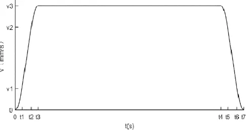
S-shaped curve is named for its shape similar to S-shaped curve in acceleration and deceleration stage. It is a commonly used speed control algorithm in current controllers. The acceleration and deceleration process of S-shaped curve is divided into seven stages, as shown in the following figure: 𝑡₀− 𝑡₁in acceleration stage, 𝑡₁ − 𝑡₂in uniform acceleration stage, 𝑡₂− 𝑡₃in deceleration stage, 𝑡₃ − 𝑡₄ in uniform acceleration stage, 𝑡₄ − 𝑡₅ in acceleration and deceleration stage, 𝑡₅− 𝑡₆ in uniform deceleration stage and 𝑡₆− 𝑡₇ in deceleration stage.

Figure 2. S-shape velocity curve.

From the definition, it can be seen that the time of acceleration change in seven segments has the following relationship:

𝑡𝑗 = 𝑡1− 𝑡0 = 𝑡3 − 𝑡2 = 𝑡5− 𝑡4 = 𝑡7− 𝑡6 𝑡_𝑎 = 𝑡₂− 𝑡₁ = 𝑡₆− 𝑡₅

𝑡_𝑣 = 𝑡₄− 𝑡₃ , (1) When 𝑡0 < 𝑡 < 𝑡1 and 𝑡0 = 0, the equations of displacement, velocity and acceleration are as follows:

𝑆(𝑡) =1₆𝐽𝑚𝑡3 V(𝑡) =1₂𝐽_𝑚𝑡2 a(𝑡) = 𝐽𝑚𝑡

. (2)

When𝑡₁ < 𝑡 < 𝑡₂, the equations of displacement, velocity and acceleration are as follows:

𝑆(𝑡) =1₂𝐽_𝑚𝑡_𝑗(𝑡 − 𝑡₁)2_{+ 𝑉(𝑡}

1)(𝑡 − 𝑡1) + 𝑋(𝑡1) 𝑉(𝑡) = 𝐽_𝑚𝑡_𝑗(𝑡 − 𝑡1) + 𝑉(𝑡1) 𝑎(𝑡) = 𝐽𝑚𝑡𝑗

. (3)

When𝑡2 < 𝑡 < 𝑡3 the equations of displacement, velocity and acceleration are as follows:

𝑆(𝑡) = −1₆𝐽𝑚𝑡𝑗(𝑡 − 𝑡2)3+₂1𝑎(𝑡2)(𝑡 − 𝑡2)2+ 𝑉(𝑡2)(𝑡 − 𝑡2) + 𝑋(𝑡2) 𝑉(𝑡) = −1₂𝐽_𝑚𝑡_𝑗(𝑡 − 𝑡2)2+ 𝑎(𝑡2)(𝑡 − 𝑡2) + 𝑉(𝑡2) 𝑎(𝑡) = −𝐽𝑚(𝑡 − 𝑡2) + 𝑎(𝑡2)

. (4)

From this we can see that the velocity of each inflection point is:

𝑉(𝑡1) =1₂𝐽𝑚𝑡12 𝑉(𝑡2) = 𝐽𝑚𝑡𝑗𝑡𝑎+1₂𝐽𝑚𝑡𝑗2 𝑉(𝑡₃) = −1₂𝐽_𝑚𝑡_𝑗2_{+ 𝐽}

𝑚𝑡𝑗2 + 𝑉(𝑡2) = 𝐽𝑚𝑡𝑗2+ 𝐽𝑚𝑡𝑗𝑡𝑎

,

Then the maximum velocity at 𝑡₃ is the maximum velocity and the maximum velocity is:

𝑉_𝑚 = 𝑉(𝑡₃) = 𝐽𝑚𝑡𝑗2 + 𝐽𝑚𝑡𝑗𝑡𝑎. (5) According to the symmetry of S-shaped curve, the expression of distance L is as follows:

𝐿 = 2𝑋(𝑡3) + 𝑆(𝑡𝑣). (6) In the formula, S(𝑡𝑣)represents the displacement in the uniform stage, and the velocity in the uniform stage is the maximum velocity 𝑉_𝑚 in the whole operation process. So the duration 𝑡_𝑣 of uniform motion is:

𝑡𝑣 = 𝐿 − (2𝐽𝑚𝑡𝑗3 + 3𝐽𝑚𝑡𝑗2𝑡𝑎+ 𝐽𝑚𝑡𝑗𝑡𝑎2) 𝑉⁄ 𝑚. (7) In summary, the relationship between distance L and 𝐽_𝑚、𝑡_𝑗、𝑡_𝑎、𝑡_𝑣 is as follows:

𝐿 = 𝐽_𝑚(2𝑡_𝑗3 _{+ 3𝑡}

𝑗2𝑡𝑎+ 𝑡𝑗𝑡𝑎2+ 𝑡𝑗2𝑡𝑣+ 𝑡𝑗𝑡𝑎𝑡𝑣). (8)

Sinusoidal Acceleration and Deceleration Curve

𝑎(𝑡) = {

𝑎𝑚𝑠𝑖𝑛𝜔𝑡 0 ≤ 𝑡 ≤ 𝑡1 0 𝑡1 ≤ 𝑡 ≤ 𝑡2 −𝑎𝑚𝑠𝑖𝑛𝜔𝑡 𝑡2 ≤ 𝑡 ≤ 𝑡3

. (9)

Among them, 𝜔 is the undetermined coefficient, 𝑡₁ is the end time of sinusoidal acceleration, and 𝑡₂ is the start time of sinusoidal deceleration.

The velocity equation can be obtained by integrating the acceleration equation (9):

𝑣(𝑡) = {

𝑎_𝑚(1 − 𝑐𝑜𝑠𝜔𝑡) 𝜔⁄ 0 ≤ 𝑡 ≤ 𝑡₁ 𝑣_𝑚 𝑡₁ ≤ 𝑡 ≤ 𝑡₂ 𝑎_𝑚[1 + 𝑐𝑜𝑠𝜔(𝑡 − 𝑡₂)] 𝜔⁄ 𝑡₂ ≤ 𝑡 ≤ 𝑡₃

. (10)

Among them, 𝑣_𝑚 is the maximum velocity.

The displacement equation can be obtained by integrating the velocity equation (10):

𝑠(𝑡) =

{

𝑎_𝑚(𝑡 − 𝑠𝑖𝑛𝜔𝑡/𝜔) 𝜔⁄ 0 ≤ 𝑡 ≤ 𝑡1 𝑆₁+ 𝑣_𝑚(𝑡 − 𝑡1) 𝑡1 ≤ 𝑡 ≤ 𝑡2

𝑆₁+ 𝑆₂+ 𝑎𝑚(𝑡 − 𝑡2) −

𝑠𝑖𝑛𝜔(𝑡−𝑡2)

𝜔 ⁄ 𝑡_𝜔

2 ≤ 𝑡 ≤ 𝑡3

. (11)

Among them, 𝑆₁ = 𝑎𝑚_𝜔𝑡1, 𝑆₂ = 𝑣_𝑚(𝑡₂− 𝑡₁),

By definition: ω𝑡₁ = 𝜋, and t = 𝑡₁,

𝜔 =2𝑎𝑚 𝑣𝑚, 𝑡1 =

𝜋 𝜔 =

𝜋𝑣𝑚 2𝑎𝑚, 𝑆1 =

𝜋𝑣𝑚2 4𝑎𝑚,

Critical state: 𝑡₁ = 𝑡₂, i.e. non-uniform stage, at which the maximum velocity 𝑣_𝑠𝑒𝑡 obtained satisfies 𝑆₁ = 𝐿₂,

Then: 𝑣_𝑠𝑒𝑡2 = 2𝑎_𝜋𝑚𝐿

.

According to the symmetry of sinusoidal acceleration and deceleration motion, we can see that:

𝑇 = 2𝑡₁+𝐿−2𝑆1

𝑣𝑚 , 𝑡2 = 𝑇 − 𝑡1.

Finally, the relationship between total displacement, velocity and planning time can be obtained：

𝑇 = 𝑡1+_𝑣𝐿

𝑚. (13) In the formula, T is the total running time.

Quintic Function Curve

Displacement equation:

𝑆(𝑡) = 𝑘5𝑡5+ 𝑘4𝑡4+ 𝑘3𝑡3+ 𝑘2𝑡2 + 𝑘1𝑡 + 𝑘0,

{

𝑘₀ = 𝑥₀ 𝑘1 = 𝑣0 𝑘2 = 𝑎0⁄ 2 𝑘3 = (20𝑥1− 20𝑥0 − 8𝑣1𝑇 − 12𝑣0𝑇 − 3𝑎0𝑇2+ 𝑎1𝑇2) (2𝑇⁄ 3) 𝑘₄ = (30𝑥₁− 30𝑥₀ + 14𝑣₁𝑇 + 16𝑣₀𝑇 + 3𝑎₀𝑇2_{− 2𝑎}

1𝑇2) (2𝑇⁄ 4) 𝑘5 = (12𝑥1− 12𝑥0 − 6𝑣1𝑇 − 6𝑣0𝑇 − 𝑎0𝑇2+ 𝑎1𝑇2) (2𝑇⁄ 5)

Among them, 𝑥₀and 𝑥₁ are the starting and ending speed, 𝑎₀ and 𝑎₁ are the starting and ending acceleration, and T is the total running time; 𝑡 ∈ [0, 𝑇].

Constraint 𝑆(𝑇) = 𝐿，𝑆′_{(0) = 0，𝑆}′_{(𝑇) = 0，𝑆}"_{(0) = 0，𝑆}"_{(𝑇) = 0.} Formula (14) can be changed to

{

𝑘₀ = 0 𝑘₁ = 0 𝑘₂ = 0 𝑘₃ =10𝐿_𝑇3 𝑘4 = −15𝐿_𝑇4 𝑘₅ =_𝑇6𝐿₅

,

Then the displacement equation of the quintic function is:

𝑆(𝑡) =10𝐿_𝑇3 𝑡3₋15𝐿 𝑇4 𝑡4+

6𝐿

𝑇5𝑡5. (15)

Simulation Analysis

The truss robot is modeled by NX three-dimensional software. The movement of X and Y direction is accomplished by servo motor with reducer as power system and gear rack as transmission system respectively. The total length of X direction is 12m, and the total span of Y direction is 8m. In actual working conditions, the displacements of X direction and Y direction are 7.68m and 3.78m respectively, and the total running time is 10s.

In order to compare the influence of three speed control methods on the smooth operation of truss robots, the three-dimensional model is imported into ADAMS software for simulation analysis and comparison. Adding gear pairs and corresponding motion in XY direction respectively, the control function of motion is completed by new SPLINE text. Since the model imported directly is a pure rigid body model, only one motion function in X direction is retained. According to the above analysis, the velocity (or displacement) equations of the three speed control modes are as follows:

1) S-shaped curve: X direction:

𝑣(𝑡) =

{

2𝑡2 _{0 ≤ 𝑡 ≤ 0.3} 0.18 + 1.2(𝑡 − 0.3) 0.3 ≤ 𝑡 ≤ 0.7 0.66 + 1.2(𝑡 − 0.7) − 2(𝑡 − 0.7)2 _{0.7 ≤ 𝑡 ≤ 1} 0.84 1 ≤ 𝑡 ≤ 9 0.84 − 2(𝑡 − 9)2 _{9 ≤ 𝑡 ≤ 9.3} 0.66 − 1.2(𝑡 − 9.3) 9.3 ≤ 𝑡 ≤ 9.7 0.18 − 1.2(𝑡 − 9.7) + 2(𝑡 − 9.7)2 _{9.7 ≤ 𝑡 ≤ 10}

,

Y direction:

𝑣(𝑡) =

{

𝑡2 _{0 ≤ 𝑡 ≤ 0.3} 0.09 + 0.6(𝑡 − 0.3) 0.3 ≤ 𝑡 ≤ 0.7 0.33 + 0.6(𝑡 − 0.7) − (𝑡 − 0.7)2 _{0.7 ≤ 𝑡 ≤ 1} 0.42 1 ≤ 𝑡 ≤ 9 0.42 − (𝑡 − 9)2 _{9 ≤ 𝑡 ≤ 9.3} 0.33 − 0.6(𝑡 − 9.3) 9.3 ≤ 𝑡 ≤ 9.7 0.09 − 0.6(𝑡 − 9.7) + (𝑡 − 9.7)2 _{9.7 ≤ 𝑡 ≤ 10} .

𝑣(𝑡) = {0.42(1 − 𝑐𝑜𝑠𝜋𝑡) 0 ≤ 𝑡 ≤ 10.84 1 < 𝑡 ≤ 9 0.42[1 + cos π(𝑡 − 9)] 9 < 𝑡 ≤ 10

,

Y direction:

𝑣(𝑡) = {0.21(1 − 𝑐𝑜𝑠𝜋𝑡) 0 ≤ 𝑡 ≤ 10.42 1 < 𝑡 ≤ 9 0.21[1 + cos π(𝑡 − 9)] 9 < 𝑡 ≤ 10

.

3) Quintic function curve: X direction:

𝑆(𝑡) = 4.536 × 10−4_{× 𝑡}5_{− 1.134 × 10}−2_{× 𝑡}4_{+ 7.56 × 10}−2_{× 𝑡}3 _{0 ≤ 𝑡 ≤ 10,} Y direction:

𝑆(𝑡) = 2.268 × 10−4_{× 𝑡}5_{− 0.567 × 10}−2_{× 𝑡}4_{+ 3.78 × 10}−2_{× 𝑡}3 _{0 ≤ 𝑡 ≤ 10.} The results of ADAMS simulation are as follows:

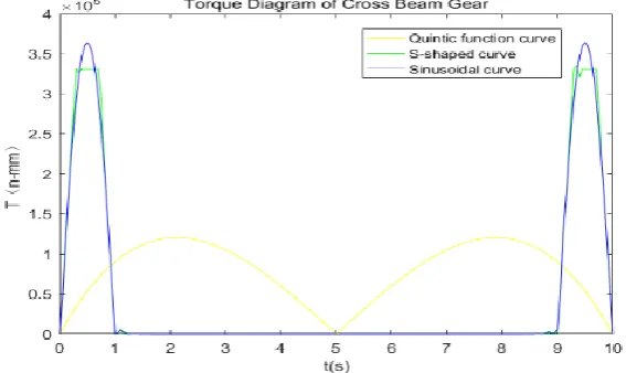
Figure 3 shows the output torque diagram of the cross-beam gear. By measuring the torque of the cross-beam gear and utilizing the transmission ratio relationship, the actual output torque of the motor and the power of the motor can be deduced. It can be seen from the graph that the required torque of truss robot motor is reduced by one third by using quintic function speed curve control mode. In the first five seconds, the acceleration increases first and then decreases, which leads to the increase and then decreases of the torque. In the second five seconds, the acceleration is negative, and the change mode is the same as the first five seconds, but the motor is in the deceleration state, and the deceleration setting is carried out through the built-in brake.

Figure 3. Torque figure of cross-beam gear.

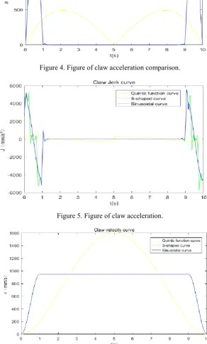
Figure 4. Figure of claw acceleration comparison.

Figure 5. Figure of claw acceleration.

Figure 6. Figure of claw velocity.

Summary

Acknowledgement

This research was financially supported by the National Natural Science Foundation of China. (Projection No. 51475311)

Reference

[1] Yang Chao, Zhang Dongquan. Acceleration and deceleration control of stepping motor based on S-curve [J]. Mechatronics Engineering, 2011, 28 (7): 813-817.

[2] You Wenhui, Wang Xiufeng, Lu Wenqi, et al. Design of trajectory planning interpolation system for industrial manipulators [J]. Mechatronics Engineering, 2019, 36 (2): 190-196.

[3] Zhang Li, Yang Dongsheng, Wang Yunsen, et al. NURBS interpolation forward-looking control algorithm based on cubic polynomial acceleration and deceleration [J]. Modular machine tools and automation processing technology, 2014 (3): 1-8.

[4] Li Hongbin, Xu Yichen, Lu Zhan. Trajectory optimization of packing and palletizing robot based on S-curve [J]. Packaging Engineering, 2018, 39 (17): 187-191.

[5] Pan Haihong, Yang Wei, Chen Lin, et al. Adaptive piecewise NURBS curve interpolation algorithm for acceleration and deceleration control of full S-curve [J]. China Mechanical Engineering, 2010, 21 (2): 190-195.

[6] Mu Haihua, Zhou Yunfei, Yan Sijie, et al. Research on 4-order trajectory planning algorithm for Ultra-precision point-to-point motion [J]. China Mechanical Engineering, 2007, 18 (19): 2346-2354.

[7] Du Qiaolian, Chen Xuhui, Shu Baihe. An improved trajectory planning method for robots [J]. Mechanical design, 2017, 34 (3): 31-35.

[8] Zhang Bin, Fang Qiang, Colin. Optimal time trajectory planning for large rigid body attitude adjustment system [J]. Journal of Mechanical Engineering, 2008, 44(8): 248-252.

[9] Haddad M, Khalil W, Lehtihet H E. Trajectory Planning of Unicycle Mobile Robots with a Trapezoidal-velocity Constraint [J]. IEEE Transactions on Robotics, 2010, 26 (5): 954-962.

[10] Peng Fang, Li Ping, Zhou Wenhui. Research on multi-axis path planning of rectangular coordinate manipulator [J]. Modular machine tools and automatic processing technology, 2012 (7): 71-74.

[11] Fu Yunzhong, Wang Yongzhang, Fu hongya, et al. Multi-axis linear interpolation and its "S acceleration and deceleration" programming algorithm [J]. Manufacturing Technology and Machine Tools, 2003, 11 (3): 375-382.