Identification of the pollution source of a parabolic equation with the time dependent heat conduction

R E S E A R C H

Open Access

Identification of the pollution source of a

parabolic equation with the time-dependent

heat conduction

Nguyen Huy Tuan

_{, Dang Duc Trong}

_{, Ta Hoang Thong}

_{and Nguyen Dang Minh}

*_{Correspondence:}

[email protected]

1_{Saigon Institute for Computational}

Science and Technology, Ho Chi Minh City, Vietnam

2_{Department of Mathematics,}

University of Natural Science, Vietnam National University, 227 Nguyen Van Cu, Distric 5, Ho Chi Minh City, Vietnam

Full list of author information is available at the end of the article

Abstract

We consider the problem of identifying the pollution source of a 1D parabolic equation from the initial and the final data. The problem is ill posed and regularization is in order. Using the quasi-boundary method and the truncation Fourier method, we present two regularization methods. Error estimates are given and the methods are illustrated by numerical experiments.

1 Introduction

In this paper, we consider an inverse problem of identifying a pollution source from data measured at some points in a watershed. The pollution source causes water contamination in some region. In all industrial countries, groundwater pollution is a serious environmen-tal problem that puts the whole ecosystem, including humans, in jeopardy. The quality and quantity of groundwater have much effect on human life and may lead to natural environ-mental changes (see,e.g., []). As we know, most efforts to find pollutant transport are based on the methodology of mathematics. Solute transport in a uniform groundwater flow can be described by the one-dimensional (D) linear parabolic equation

∂u˜ ∂t –D

∂u˜ ∂x +V

∂u˜

∂x+Ru˜=F(x,t), x∈,  <t<T, ()

whereis a spatial domain,u˜ is the solute concentration,V represents the velocity of watershed movement,Rdenotes the self-purifying function of the watershed, andF(x,t) is a source term causing the pollution functionu˜(x,t). Putting

˜

u(x,t) =u(x,t)eVDx–(V

 D+R)t_,

we can transform the latter equation into

∂u ∂t –D

∂u

∂x =F(x,t), ()

whereF(x,t) =F(x,t)e–

V

Dx+(V



D+R)t_{; we still call it the source function. Coming from this} relationship between the two equations () and (), in the present paper, we will find a pair

of functions (u,F) satisfying () subject to the initial and the final conditions

u(x, ) = , u(x,T) =g(x), x∈(,π), ()

and the boundary conditionu(,t) =u(π,t) = . To consider a more general case, we will replaceDin () by a given functiona(t) which is defined later.

This inverse source problem is ill posed. Indeed, a solution corresponding to the given data does possibly not exist, and even if the solution exists (uniquely) then it may not depend continuously on the data. Because the problem is severely ill posed and difficult, many preassumptions on the form of the heat source are in order. In fact, let{ϕn(t)}be a

basis inL_{(,T). Then the functionFcan be written as}

F(ξ,t) = ∞

n=

ϕn(t)fn(ξ). ()

In the simplest case, one reduces this approximation to its first termF(x,t) =ϕ(t)f(x), where the functionϕis given. Source terms of this form frequently appear, for example, as a control term for the parabolic equation.

In another context, this problem is called the identification of heat source; it has received considerable attention from many researchers in a variety of fields using different methods since . If the pollute source has the form off =f(u), the inverse source problem was studied in []. In [], the authors considered the heat source as a function of both space and time variables, in the additive or separable forms. Many researchers viewed the source as a function of space or time only. In [, ], the authors determined the heat source dependent on one variable in a bounded domain by the boundary-element method and the iterative algorithm. In [], the authors investigated the heat source which is time-dependent only by the method of a fundamental solution.

Many authors considered the uniqueness and stability conditions of the determination of the heat source under this separate form. In spite of the uniqueness and stability results, the regularization problem for unstable cases is still difficult. For a long time, it has been investigated for a heat source which is time-depending only [, , ] or space-depending only [, , –]. As regards the regularization method, there are few papers with a strict theoretical analysis of identifying the heat sourceF(x,t) =ϕ(t)f(x), whereϕis a given func-tion. Tronget al.[, ] considered this problem by the Fourier transformation method. Recently, whena(t) =  andϕ(t) =e–λt_{(λ> ), the problem () describes a heat process of}

radio isotope decay whose decay rate isλ, which has been considered by Qian and Li []. In [], Hasanov identified the heat source which has the form ofF(x,t) =F(x)H(t) of the variable coefficient heat conduction equationut = (k(x)ux)x+F(x)H(t) using the

varia-tional method. However, the generalized case with the time-dependent coefficient ofu

in the main equation is still limited and open. In this paper, we consider the following generalized equation:

ut–a(t)uxx=F(x,t) ()

pollution source identification problems (see []). Such a model is related to the detection of the pollution source causing water contamination in some region.

The remainder of the paper is divided into three sections. In Section , we apply the quasi-boundary value method and truncation method to solve the problem ()-(). Then we also estimate the error between an exact solution and the regularization solution with the logarithmic order and Hölder order. Finally, some numerical experiments will be given in Section .

2 Identification and regularization for inhomogeneous source depending on time variable

Let · ,·,·be the norm and the inner product inL(,π). Leta: [,T]→Rbe a con-tinuous function on [,T]. We setA(t) =_ta(s)ds. The problem () can be transformed into

⎧ ⎪ ⎨ ⎪ ⎩

d

dtu(x,t),sinnx+n

_{a(t)u(x,t),sinnx=ϕ(t)f(x),sinnx,  <t<T,}

u(x,t),sinnx= ,

u(x,T),sinnx=g(x),sinnx.

()

By an elementary calculation, we can solve the ordinary differential equation () to get

f(x),sinnx =enA(T)

T



enA(t)ϕ(t)dt –

g(x),sinnx

or

f(x) = ∞

n=

enA(T)

T



enA(t)_ϕ(t)dt –

gnsinnx, ()

where gn= πg(x),sinnx. Note that en _A(T)

increases rather quickly whenn becomes large. Thus the exact data function g(x) must satisfy the property that g(x),sinnx de-cays rapidly. But in applications, the input datag(x) can only be measured and never be exact. We assume the data functionsg (x)∈L_{(,π),ϕ,ϕ ∈L}_{(,T) to satisfy}

g –g≤ , ϕ –ϕ ≤ ()

andϕ(t) >C, ϕ (t) >C, t∈(,T), where the constant represents a noise level and

C> .

Lemma  Let s> ,X≥.Then for all≤t≤T and < < ,we have

( +X)s_{( +e}–TX₎≤s

s_e–s_{ +T}–s T

ln(/ )

s

. ()

Proof Case.X∈[,_T]. It is clear to see that

( +X)s_{( +e}–TX₎≤_{( +X)}s_e–TX ≤ e

From the inequality ≤(s_e)s₍ 

ln(/))s, we get

( +X)k_{( +e}–TX₎≤s s_e–s



ln(/ )

s

≤sse–s +T–s T ln(/ )

s

.

Case.X>_T. Sete–TX= Y. Then we obtain

( +X)s_{( +e}–TX₎= _{+ Y}

T T–ln( Y)

s

= 

 +Y

T T–ln( Y)

s

= 

 +Y

T ln(/ )

s

–ln( )

T–ln( Y)

s

=

T ln(/ )

s

  +Y

–ln( )

T–ln( Y)

s

.

We continue to estimate the term _+_Y(_T–_–lnln(_(Y)₎)s_.

If  <Y≤ then  < –ln( ) < –ln( Y), thus

  +Y

–ln( )

T–ln( Y)

s

< ,

else ifY>  thenlnY>  andln( Y) = –TX< – due to the assumptionX∈(_T,∞). There-fore,lnY( +ln( Y))≤. This implies that

 < –ln

T–ln( Y)< –ln

–ln( Y)<  +lnY. ()

Hence, in this case, we get

  +Y

–ln( )

T–ln( Y)

s

<( +lnY)

s

Y = ( +lnY)

s_Y–_{. ()}

Setg(Y) = ( +lnY)s_Y–_forY>e–_{. Taking the derivative of this function, we get}

g(Y) = ( +lnY)s–_Y–_{(s–  –lnY). ()}

The functionghas a maximum at the pointY, so thatg(Y) = . This implies thatY=

es–_{. Therefore}

sup

Y≥

( +lnY)s_Y–_≤g(Y

) =sse–s. ()

Since (), (), we have

  +Y

–ln( )

T–ln( Y)

s

From (), we get

( +X)s_{( +e}–TX₎≤s s_e–s

T ln(/ )

s

≤sse–s +T–s T ln(/ )

s

.

Lemma  Let a: [,T]→R be a continuous function on[,T].Let p=inf_≤t≤Ta(t),q=

sup_≤t≤Ta(t).Then we have

(i)

T

 exp

n

t



a(s)ds

dt –

≤ 

T, ()

(ii) 

( +n₎k_{(α( ) +e}–n_A(T)

)≤

B(q,k,T)

α( )

_ln(qT

α())

k, ()

where

B(q,k,T) =kke–k + (qT)–k_.

Proof (i) Sincea(t)≥p, we have

T

 exp

n

t



a(s)ds

dt –

= _T 

 exp(n t

a(s)ds)dt

≤T 

 exp(n t

p ds)dt

= _T   epn

_t dt=

pn

epn_T

– ≤ 

T. ()

(ii) Sincea(t)≤q, we gete–nA(T)≥e–nqT. Then using Lemma , we get 

( +n₎k_{(α( ) +e}–n_A(T)

)≤



( +n₎k_{(α( ) +e}–n_qT

)

≤ B(q,k,T)

α( )

_ln(qT

α())

k. ()

2.1 Regularization by a quasi-boundary value method

Denote by · kthe norm in Sobolev spaceHk(,π) defined by

fk=

_∞

n=

 +nk|fn|

 

,

wherefn=πf(x),sinnx.

We modify the problem ()-() by perturbing the Fourier expansion of final valuegas follows:

⎧ ⎪ ⎪ ⎪ ⎪ ⎨ ⎪ ⎪ ⎪ ⎪ ⎩

∂u

∂t –

∂ ∂x(a(t)

∂u

∂x) =ϕ (t)f (x), x∈(,π),  <t<T,

u (x, ) = , x∈(,π),

u (,t) =u (π,t) = , t∈(,T),

u (x,T) =_n∞_= e–A(T)n



α( )+e–A(T)ngnsinnx, x∈(,π),

whereg_n=_πg (x),sinnxandα( ) is a regularization parameter such thatlim _→α( ) = . This problem is based on the quasi-boundary regularization method which is given in []. This method has been studied for solving various types of inverse problem [, ]. The solution of this problem is given by

f (x) = ∞

n=



α( ) +e–n_A(T)

T



enA(t)ϕ (t)dt –

g_nsinnx. ()

Now we will give an error estimate between the regularization solution and the exact so-lution by the following theorem.

Theorem  Suppose that f,g∈L_{(,π)such thatf}

k<∞andgk+_ <∞for some

k≥.Let g ∈L(,π)be measured data at t=T satisfying().Let f be the regularized solution given by().If we selectα( )such that

lim

→α( )= ,

thenlim →f –f= and we have following estimate:

f –f ≤

CTα( )

+C(p,q,k,T)

α( )

_ln(

α()) kgk+



+B(q,k,T) qT

ln(_α(₎)

kfk. ()

Proof We define

h (x) = ∞

n=



α( ) +e–n_A(T)

T



enA(t)_{ϕ (t)dt} –

gnsinnx ()

and

p (x) = ∞

n=



α( ) +e–n_A(T)

T



enA(t)_ϕ(t)dt –

gnsinnx. ()

We divide the proof into three steps.

Step . Estimatef –h. From () and (), we have

f –h= ∞

n=

 (α( ) +e–n_A(T)

)

T



enA(t)ϕ (t)dt –

g_n–gn



≤ ∞

n=  _ln₍qT

) 

(_TCdt)

g_n–gn



≤ _| 

α( )| 

(_TCdt)

g –g

≤ 

C

T|α( )|

Step . Estimateh –p . From (), (), and (), we have

h –p

= ∞

n=

 (α( ) +e–n_A(T)

)

T



enA(t)ϕ (t)dt –

–

T



enA(t)ϕ(t)dt –

g_n

= ∞

n=



( +n₎k_{(α( ) +e}–n_A(T)

)

(_TenA(t)(ϕ(t) –ϕ (t))dt) (_Ten_A(t)

ϕ (t)dt)₍T  en

_A(t) ϕ(t)dt)

 +nkg_n

≤B(q,k,T)

α( )

_ln(qT

α()) k∞

n=

[_TenA(t)_dt][T

 |ϕ (t) –ϕ(t)|dt] (_Ten_A(t)

ϕ(t)dt)₍T  en

_A(t)

ϕ (t)dt)

 +nkg_n

≤B(q,k,T)

α( )

_ln(qT

α()) k × ∞ n=

[_TenA(t)_dt][T

 |ϕ (t) –ϕ(t)|dt]

C_T₍T  en

_A(t) dt)

 +nk_g

n. ()

On other hand, we have

enA(T)–enA()=enA(T)–  =

T



enA(t)(t)dt

=

T



nA(t)enA(t)dt=

T



na(t)enA(t)dt.

Sincep≤a(t)≤q, we get

p T



enA(t)dt≤ T



a(t)enA(t)dt≤q T



enA(t)dt.

Hence

en_A(T)

– 

qn ≤

T



enA(t)dt≤e

n_A(T)

– 

pn . ()

It follows from () and () that

h –p

≤B(q,k,T)

α( )

_ln(qT

α()) k∞

n=

q_(enA(T)_{– )ϕ (t) –ϕ(t)} pC_T_(en_A(T)

– )

 +nk+g_n. ()

Since

enA(T)–  (en_A(T)

– ) =

 –e–nA(T)

( –e–n_A(T)

) ≤

  –e–n_A(T)



≤

  –e–A(T)



≤

  –e–pT

andϕ (t) –ϕ(t)_≤ _{, we obtain}

h –p≤ q



pC

T( –e–pT)

B(_αq₍,k₎,T)_ln(qT α())

k∞

n=

 +nk+g_n

=C(p,q,k,T)

α( )

_ln(

α( ))

kgk+ 

.

Here

C(p,q,k,T) = q

√pC_T_{( –e}–pT₎B(q,k,T)(qT) k_.

Hence

h –p ≤C(p,q,k,T)

α( )

_ln(

α( )) kgk+

 . ()

Step . Estimatep –f. In fact, using the Fourier expansion off, we have

p –f₌

∞

n=



α( ) +e–n_A(T) –e

nA(T)

 T



enA(t)_ϕ(t)dt –

g

n

= ∞

n=

α( )

α( ) +e–n_A(T) 

enA(T) T

 en _A(t)

ϕ(t)dt 

g_n

= ∞

n=

α( )

α( ) +e–n_A(T) 

f_n.

Using Lemma , we obtain

p –f= ∞

n=

|α( )| ( +n₎k_{(α( ) +e}–n_A(T)

)

 +nkf_n

≤B(q,k,T) qT

ln(  α())

kf_k.

This implies that

p –f ≤B(q,k,T) qT

ln(_α₍₎)

kfk. ()

Combining Steps , , and  and using the triangle inequality, we get

f –f ≤ f –h+h –p +p –f

≤

CTα( )

+C(p,q,k,T)

α( )

_ln(

α()) kgk+



+B(q,k,T) qT

ln(_α(₎)

kfk. ()

Remark  If we chooseα( ) = m_{,  <m< , then () holds.}

Remark  In this theorem, with the assumptionf ∈Hk_{(,π), we have an errorf –fof}

logarithmic order. In the next section, we introduce a truncation method which improves the order of the error. We present the error of Hölder estimates (the order is α_{,  <α< )}

with a weaker assumption off,i.e.,f ∈H_(,π).

2.2 Regularization by a truncation method

Theorem  Suppose that f ∈H_{(,π).Let g ∈L}_{(,π)be measured data at t=T}

satis-fying().Put

f (x) =

N

n=

enA(T)

T



enA(t)ϕ (t)dt –

g_nsinnx, ()

where N= [ k– _{] + ,k}∈_{(, ).Then the following estimate holds:}

f –f≤Q –k_{+ P} k_{, ()}

where

P=



C 

+ q

_g pC

( –e–pT) ,

Q=

√π+

π



f_H_(,π).

Proof From () and (), we have

f(x) –f (x)

= ∞

n=

enA(T) T

 en _A(t)

ϕ(t)dtgn sinnx–

N

n=

enA(T) T

 en _A(t)

ϕ (t)dtgn sinnx

= ∞

n=N+

en_A(T) T

 en _A(t)

ϕ(t)dtgnsinnx+

N

n=

en_A(T) T

 en _A(t)

ϕ(t)dtgnsinnx

–

N

n=

enA(T) T

 en _A(t)

ϕ (t)dtgn sinnx

=I+I, ()

where

I=

∞

n=N+

enA(T) T

 en _A(t)

ϕ(t)dtgnsinnx ()

and

I=

N

n=

enA(T) T

 en _A(t)

ϕ(t)dtgn sinnx–

N

n=

enA(T) T

 en _A(t)

ϕ (t)dtgn

Step . We estimateI. In fact, since (), we get

I=

∞

n=N+

enA(T) (_Ten_A(t)

ϕ(t)dt)g 

n=

∞

n=N+

f_n. ()

Using integration by parts, we have

fn=

π



f(x)sinnx dx= –cosnx

n f(x) x=π

x= +

n π



f(x)cosnx dx

=

nf() –

(–)n

n f(π) +



n π



f(x)cosnx dx. ()

Hence

|fn| ≤|

f()|+|f(π)|

n +

π

 

nf

_{(x). ()}

On the other hand, sinceH(,π) is embedded continuously inC[,π] we can assume thatu∈C[,π]. So, there exists anm∈[,π] such thatf(m) = 

π π

 f(x)dx. We have

f(π) =f(m) +

π

m

f(x)dx,

f() =f(m) –

m



f(x)dx.

()

It follows that

f(π)≤f(m)+

π

m

f(x)dx≤  π

π



f(x)dx+

π



f(x)dx

≤

π

π



_f(x)

+f(x)dx=√πfH_(,π). ()

In a similar way, we also obtain|f()| ≤√πfH_(,π). Hence|f_n| ≤ 

√

π+√π_

n fH_(,π).

This implies that

I≤

∞

n=N+

(√π+π )



n f



H_(,π)

≤

√π+

π





f

H_(,π)

∞

n=N+ 

n_–n

≤

√π+

π





f_H_(,π)



N. ()

Step . We estimateI. The term () can be rewritten as follows:

I=

N

n=

enA(T)_[g

n

T

 en _A(t)

ϕ (t)dt–g_nTenA(t)_ϕ(t)dt] (_Ten_A(t)

ϕ(t)dt)(_Ten_A(t)

ϕ (t)dt) sinnx

=

N

n=

enA(T)_[(g

n–gn)

T

 en _A(t)

ϕ (t)dt+gn

T

 en _A(t)

(ϕ (t) –ϕ(t))dt]

(_Ten_A(t)

ϕ(t)dt)(_Ten_A(t) ϕ (t)dt)

Then

I≤

N

n=

enA(T)_(g

n–gn)

(_Ten_A(t)

ϕ(t)dt) + 

N

n=

en_A(T) g

n[

T

 e

n_A(t)

(ϕ (t) –ϕ(t))dt]

(_Ten_A(t)

ϕ(t)dt)₍T  en

_A(t)

ϕ (t)dt). ()

Using en

_A(T) –

qn ≤ T

 en _A(t)

dt, we have

N

n=

enA(T)_(g

n–gn)

(_Ten_A(t)

ϕ(t)dt) ≤

N

n=

enA(T)

C_(_Ten_A(t) dt)

gn–gn



≤

N

n=

nqenA(T) C

(en _A(T)

– )

gn–gn



≤

N

n=

n_q

C_( –e–n_A(T)

)

gn–gn



≤Nq 

C

. ()

In a similar way and using (), we also obtain

N

n=

enA(T)g_n[_TenA(t)(ϕ (t) –ϕ(t))dt] (_Ten_A(t)

ϕ(t)dt)₍T  en

_t

ϕ (t)dt)

≤

N

n=

enA(T)_g

n[

T

 en _A(t)

dt][_T|ϕ (t) –ϕ(t)|_dt] (_Ten_A(t)

ϕ(t)dt)₍T  en

_A(t)

ϕ (t)dt)

≤

N

n=

enA(T)_g

nq[

T

 en _A(t)

dt][_T|ϕ (t) –ϕ(t)|_dt]

C_(_Ten_A(t) dt)

≤

N

n=

nqenA(T)(enA(T)– )g_n 

pC (en

_A(T)

– )

≤

N

n=

n_q_{( –e}–nA(T)_)g

n 

pC_( –e–n_A(T)

) . ()

It is easy to see that  –e–nA(T)≤



–e–pT. It implies that

N

n=

enA(T)_g

n[

T

 en _A(t)

(ϕ (t) –ϕ(t))dt]

(_Ten_A(t)

ϕ(t)dt)₍T  en

_A(t)

ϕ (t)dt)

≤

N

n=

Ng_n 

C

( –e–pT)

≤ Nq  pC_( –e–pT₎

∞

n=

g_n

≤ Nq g

Therefore

I≤ N 

C

+ N

_q _g pC( –e–pT)

≤N P,

whereP=



C_ +

q_g

pC_(–e–pT₎. Hence

I ≤N P. ()

Combining (), (), and (), we obtain

f–f =I+I ≤ I+I

≤

√π+

π



fH_(,π)



N+PN

 _{. ()}

SinceN= [ k– _{] + , we obtain}

f–f ≤Q –k _{+ P} k_{, ()}

whereQ= (√π+π_)fH_(,π).

3 Numerical results

In this section, we consider some examples simulation for the theory in Section . In nu-merical experiments, we are interested in the error between exact source and source with approximation as RMSE:

RMSE(f,f ) := 

N

N

n=

f(xn) –f (xn)



withf(xn),f (xn) a discretization of functionf,f .

Now, we consider

⎧ ⎪ ⎨ ⎪ ⎩

ut–a(t)uxx=ϕ(t)f(x), x∈(,π),t∈(, ),

u(,t) =u(π,t) = , t∈(, ),

u(x,T) =g(x), x∈(,π),

where

a(t) =t+ ,

ϕ(t) =t+t+ ,

g(x) =sinx.

We can see the exact source

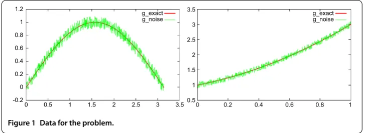
Using FORTRAN , we have a generator for noise data from routinerand() which is a random variable with the uniform distribution on [, ]. Therefore, we have measurement data with noise

g (x) =sinx+ ∗rand(),

ϕ (t) =t+t+  + ∗rand(),

where = –r_{, withr= , , , , works as the amplitude of noise.}

We can easily see

g–g < √π, φ–φ < √π

and we have convergence to zero.

From Figure , we can compare between exact data and measured data.

We consider the source approximation with the quasi-reversibility regularization

f (x) = ∞

n=





enA(t)ϕ (t)dt –

g_nsinnx

+e–n_A().

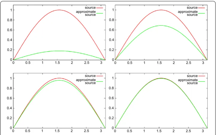
We have the table of errors with = –_{, }–_{, }–_{and }–_{(see Table ) and Figure .} On the other hand, we have the source approximation with the truncation Fourier reg-ularization

f (x) =

N

n=





enA(t)ϕ (t)dt –

enA()g_nsinnx.

We have the table of errors = –, –, –and –(see Table ) and Figure  is as in Table .

Figure 1 Data for the problem.

Table 1 The error estimation between exact solution and regularized solution by quasi-reversibility method

10–1 ₁₀–2 ₁₀–3 ₁₀–4

Figure 2 The approximation source.Red is for the exact solution and green is for the approximation from the quasi-reversibility regularization.

Table 2 The error estimation between exact solution and regularized solution by truncation method

10–1 ₁₀–2 ₁₀–3 ₁₀–4

RMSE(f,f ) 1.74326×10–2 _4.3520810–4 _1.38719–5 _5.67552–6

Figure 3 The approximation source.Red is for the exact solution and green is for the approximation from the truncation Fourier regularization.

Competing interests

Authors’ contributions

All authors contributed equally to the writing of this paper. All authors read and approved the final manuscript.

Author details

1_{Saigon Institute for Computational Science and Technology, Ho Chi Minh City, Vietnam.}2_{Department of Mathematics,}

University of Natural Science, Vietnam National University, 227 Nguyen Van Cu, Distric 5, Ho Chi Minh City, Vietnam.

3_{High School for the Gifted, Vietnam National University, Ho Chi Minh City, Vietnam.}

Acknowledgements

This research is funded by the Institute for Computational Science and Technology at Ho Chi Minh City (ICST HCMC) under the project name ‘Inverse parabolic equation and application to groundwater pollution source’.

Received: 30 January 2014 Accepted: 25 March 2014 Published:06 May 2014

References

1. Atmadja, J, Bagtzoglou, AC: Marching-jury backward beam equation and quasi-reversibility methods for hydrologic inversion: application to contaminant plume spatial distribution recovery. Water Resour. Res.39, 1038-1047 (2003) 2. Cannon, JR, Duchateau, P: Structural identification of an unknown source term in a heat equation. Inverse Probl.14,

535-551 (1998)

3. Savateev, EG: On problems of determining the source function in a parabolic equation. J. Inverse Ill-Posed Probl.3, 83-102 (1995)

4. Farcas, A, Lesnic, D: The boundary-element method for the determination of a heat source dependent on one variable. J. Eng. Math.54, 375-388 (2006)

5. Johansson, T, Lesnic, D: Determination of a spacewise dependent heat source. J. Comput. Appl. Math.209, 66-80 (2007)

6. Yan, L, Fu, C-L, Yang, F-L: The method of fundamental solutions for the inverse heat source problem. Eng. Anal. Bound. Elem.32, 216-222 (2008)

7. Yang, F, Fu, C-L: Two regularization methods for identification of the heat source depending only on spatial variable for the heat equation. J. Inverse Ill-Posed Probl.17(8), 815-830 (2009)

8. Cheng, W, Fu, C-L: Identifying an unknown source term in a spherically symmetric parabolic equation. Appl. Math. Lett.26, 387-391 (2013)

9. Yang, F, Fu, C-L: A simplified Tikhonov regularization method for determining the heat source. Appl. Math. Model.34, 3286-3299 (2010)

10. Yang, F, Fu, C-L: A mollification regularization method for the inverse spatial-dependent heat source problem. J. Comput. Appl. Math.255, 555-567 (2014)

11. Trong, DD, Tuan, NH: A nonhomogeneous backward heat problem: regularization and error estimates. Electron. J. Differ. Equ.2008, 33 (2008)

12. Trong, DD, Quan, PH, Alain, PND: Determination of a two dimensional heat source: uniqueness, regularization and error estimate. J. Comput. Appl. Math.191, 50-67 (2006)

13. Qian, A, Li, Y: Optimal error bound and generalized Tikhonov regularization for identifying an unknown source in the heat equation. J. Math. Chem.49(3), 765-775 (2011)

14. Hasanov, A: Identification of spacewise and time dependent source terms in 1D heat conduction equation from temperature measurement at a final time. Int. J. Heat Mass Transf.55, 2069-2080 (2012)

15. Denche, M, Bessila, K: A modified quasi-boundary value method for ill-posed problems. J. Math. Anal. Appl.301, 419-426 (2005)

10.1186/1029-242X-2014-161