Rain or snow: hydrologic processes, observations, prediction, and research needs

www.hydrol-earth-syst-sci.net/21/1/2017/ doi:10.5194/hess-21-1-2017

© Author(s) 2017. CC Attribution 3.0 License.

Rain or snow: hydrologic processes, observations,

prediction, and research needs

Adrian A. Harpold1, Michael L. Kaplan2, P. Zion Klos3, Timothy Link3, James P. McNamara4, Seshadri Rajagopal2, Rina Schumer2, and Caitriana M. Steele5

1_{Department of Natural Resources and Environmental Science, University of Nevada, 1664 N. Virginia Street,}

Reno, Nevada, USA

2_{Division of Hydrologic Sciences, Desert Research Institute, 2215 Raggio Parkway, Reno, Nevada, USA}

3_{Department of Forest, Rangeland, and Fire Sciences, University of Idaho, 875 Perimeter Drive, Moscow, Idaho, USA} 4_{Department of Geosciences, Boise State University, 1910 University Dr., Boise, Idaho, USA}

5_{Jornada Experimental Range, New Mexico State University, Las Cruces, New Mexico, USA}

Correspondence to:Adrian A. Harpold ([email protected])

Received: 23 August 2016 – Published in Hydrol. Earth Syst. Sci. Discuss.: 31 August 2016 Revised: 6 December 2016 – Accepted: 8 December 2016 – Published: 2 January 2017

Abstract. The phase of precipitation when it reaches the ground is a first-order driver of hydrologic processes in a wa-tershed. The presence of snow, rain, or mixed-phase precip-itation affects the initial and boundary conditions that drive hydrological models. Despite their foundational importance to terrestrial hydrology, typical phase partitioning methods (PPMs) specify the phase based on near-surface air tempera-ture only. Our review conveys the diversity of tools available for PPMs in hydrological modeling and the advancements needed to improve predictions in complex terrain with large spatiotemporal variations in precipitation phase. Initially, we review the processes and physics that control precipitation phase as relevant to hydrologists, focusing on the importance of processes occurring aloft. There is a wide range of op-tions for field observaop-tions of precipitation phase, but there is a lack of a robust observation networks in complex ter-rain. New remote sensing observations have the potential to increase PPM fidelity, but generally require assumptions typ-ical of other PPMs and field validation before they are oper-ational. We review common PPMs and find that accuracy is generally increased at finer measurement intervals and by in-cluding humidity information. One important tool for PPM development is atmospheric modeling, which includes mi-crophysical schemes that have not been effectively linked to hydrological models or validated against near-surface precipitation-phase observations. The review concludes by describing key research gaps and recommendations to

im-prove PPMs, including better incorporation of atmospheric information, improved validation datasets, and regional-scale gridded data products. Two key points emerge from this syn-thesis for the hydrologic community: (1) current PPMs are too simple to capture important processes and are not well validated for most locations, (2) lack of sophisticated PPMs increases the uncertainty in estimation of hydrological sen-sitivity to changes in precipitation phase at local to regional scales. The advancement of PPMs is a critical research fron-tier in hydrology that requires scientific cooperation between hydrological and atmospheric modelers and field scientists.

1 Introduction and motivation

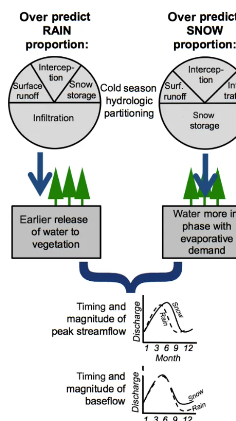
modeling in both applied and research settings. Snow stor-age delays the transfer of precipitation to surface runoff, in-filtration, and generation of streamflows (Fig. 1), affecting the timing and magnitude of peak flows (Wang et al., 2016), hydrograph recession (Yarnell et al., 2010), and the magni-tude and duration of summer baseflow (Safeeq et al., 2014; Godsey et al., 2014). Moreover, the altered timing and rate of snow versus rain inputs can modify the partitioning of water to evapotranspiration versus runoff (Wang et al., 2013). Mis-representation of precipitation phase within hydrologic mod-els thus propagates into spring snowmelt dynamics (Harder and Pomeroy, 2013; Mizukami et al., 2013; White et al., 2002; Wen et al., 2013) and streamflow estimates used in wa-ter resource forecasting (Fig. 1). The persistence of stream-flow error is particularly problematic for hydrological models that are calibrated on observed streamflows because this error can be compensated for by altering parameters that control other states and fluxes in the model (Minder, 2010; Shamir and Georgakakos, 2006; Kirchner, 2006). Expected changes in precipitation phase from climate warming presents a new set of challenges for effective hydrological modeling (Fig. 1). A simple yet essential issue for nearly all runoff generation questions is this: is precipitation falling as rain, snow, or a mix of both phases?

Despite advances in terrestrial process representation within hydrological models in the past several decades (Fatichi et al., 2016), most state-of-the-art models rely on simple empirical algorithms to predict precipitation phase. For example, nearly all operational models used by the National Weather Service River Forecast Centers in the United States use some type of temperature-based precipita-tion phase partiprecipita-tioning method (PPM) (Pagano et al., 2014). These are often single or double temperature threshold mod-els that do not consider other conditions important to the hy-drometeor’s energy balance. Although forcing datasets for hydrological models are rapidly being developed for a suite of meteorological variables, to date no gridded precipitation-phase product has been developed over regional to global scales. Widespread advances in both simulation of terres-trial hydrological processes and computational capabilities may have limited improvements on water resources forecasts without commensurate advances in PPMs.

Recent advances in PPMs incorporate effects of humid-ity (Harder and Pomeroy, 2013; Marks et al., 2013), atmo-spheric temperature profiles (Froidurot et al., 2014), and re-mote sensing of phase in the atmosphere (Minder, 2010; Lundquist et al., 2008). A challenge to improving and se-lecting PPMs is the lack of validation data. In particular, reli-able ground-based observations of phase are sparse, collected at the point scale over limited areas, and are typically lim-ited to research rather than operational applications (Marks et al., 2013). The lack of observations is particularly prob-lematic in mountain regions where snow–rain transitions are widespread and critical for regional water resource evalua-tions (Klos et al., 2014). For example, direct visual

observa-Figure 1.Precipitation phase has numerous implications for mod-eling the magnitude, storage, partitioning, and timing of water in-puts and outin-puts. Potentially affecting important ecohydrological and streamflow quantities important for prediction.

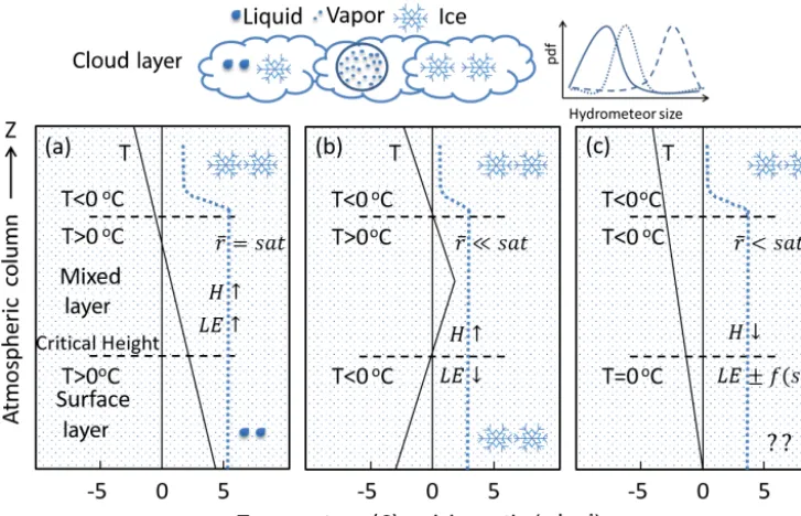
Figure 2.The phase of precipitation at the ground surface is strongly controlled by atmospheric profiles of temperature and humidity. While conditions exist that are relatively easy to predict rain(a)and snow(b), many conditions lead to complex heat exchanges that are difficult to predict with ground-based observations alone(c). The blue dotted line represents the mixing ratio.H,LE,f(sat), andrare abbreviations for sensible heat, latent heat of evaporation, function of saturation, and mixing ratio, respectively. The arrows afterH orLEindicate the energy of the hydrometeor either increasing (up) or decreasing (down), which is controlled by other atmospheric conditions.

conventional PPMs, is needed to determine critical knowl-edge gaps and research opportunities.

New efforts are needed to advance PPMs to better inform hydrological models by integrating new observations, ex-panding the current observation networks, and testing tech-niques over regional variations in hydroclimatology. While calls to integrate atmospheric information are an important avenue for advancement (Feiccabrino et al., 2013), hydrolog-ical models ultimately require accurate and validated phase determination at the land surface. Moreover, any advance-ment that relies on integrating new information or develop-ing a new PPM technique will require validation and traindevelop-ing using ground-based observations. To make tangible hydro-logical modeling advancements, new techniques and datasets must be integrated with current modeling tools. The first step towards improved hydrological modeling in areas with mixed precipitation phase is educating the scientific commu-nity about current techniques and limitations that convey the areas where research is most needed.

Our review paper is motivated by a lack of a compre-hensive description of the state-of-the-art PPMs and obser-vation tools. Therefore, we describe the current state of the science in a way that clarifies the correspondence between techniques and observations, and highlights strengths and weaknesses in the current scientific understanding. Specifi-cally, subsequent sections will review (1) the processes and physics that control precipitation phase as relevant to field

hydrologists, (2) current available options for observing pcipitation phase and related measurements common in re-mote field settings, (3) existing methods for predicting and modeling precipitation phase, and (4) research gaps that ex-ist regarding precipitation-phase estimation. The overall ob-jective is to convey a clear understanding of the diversity of tools available for PPMs in hydrological modeling and the advancements needed to improve predictions in complex ter-rain characterized by large spatiotemporal variations in pre-cipitation phase.

2 Processes and physics controlling precipitation phase Precipitation formed in the atmosphere is typically a solid in the mid-latitudes and its phase at the land surface is de-termined by whether it melts during falling (Stewart et al., 2015). Most hydrologic models do not simulate atmospheric processes and specify precipitation phase based on surface conditions alone (see Sect. 4.1), ignoring phase transforma-tions in the atmosphere.

atmospheric humidity profile (Harder and Pomeroy, 2013). The vertical temperature and humidity (represented by the mixing ratio) profile through which the hydrometeor falls typically consists of three layers, a top layer that is frozen (T <0◦C) in winter in temperate areas (Stewart, 1992), a mixed layer where T can exceed 0◦C, and a surface layer that can be above or below 0◦C (Fig. 2). The phase of pre-cipitation at the surface partly depends on the phase reaching the top of the surface layer, which is defined as the critical height. The temperature profile and depth of the surface layer control the precipitation phase reaching the ground surface. For example, in Fig. 2a, if rain reaches the critical height, it may reach the surface as rain or ice pellets depending on small differences in temperature in the surface layer (Theri-ault and Stewart, 2010). Similarly, in Fig. 2b, if snow reaches the critical height, it may reach the surface as snow if the temperature in the surface layer is below freezing. However, in Fig. 2c, when the surface layer temperatures are close to freezing and the mixing ratios are neither close to saturation nor very dry, the phase at the surface is not easily determined by the surface conditions alone.

In addition to strong dependence on the vertical tempera-ture and humidity profiles, precipitation phase is also a func-tion of fall rate and hydrometeor size because they affect en-ergy exchange with the atmosphere (Theriault et al., 2010). Precipitation rate influences the precipitation phase; for ex-ample, a precipitation rate of 10 mm h−1reduces the amount of freezing rain by a factor of 3 over a precipitation rate of 1 mm h−1(Theriault and Stewart, 2010) because there is less time for turbulent heat exchange with the hydrometeor. A solid hydrometeor that originates in the top layer and falls through the mixed layer can reach the surface layer as wet snow, sleet, or rain. This phase transition in the mixed layer is primarily a function of latent heat exchange driven by va-por pressure gradients and sensible heat exchange driven by temperature gradients. Temperature generally increases from the mixed layer to the surface layer causing sensible heat in-puts to the hydrometeor. If these gains in sensible heat are combined with minimal latent heat losses resulting from low vapor pressure deficits, it is likely that the hydrometeor will reach the surface layer as rain (Fig. 2). However, vapor pres-sure in the mixed layer is often below saturation leading to latent energy losses and cooling of the hydrometeor coupled with diabatic cooling of the local atmosphere, which can pro-duce snow or other forms of frozen precipitation at the sur-face even when temperatures are above 0◦C. Likewise, sur-face energetics affect local atmospheric conditions and dy-namics, especially in complex terrain. For example, melting of the snowpack can cause diabatic cooling of the local at-mosphere and affect the phase of precipitation, especially when air temperatures are very close to 0◦C (Theriault et al., 2012). Many conditions lead to a combination of latent heat losses and sensible heat gains by hydrometeors (Fig. 2). Un-der these conditions it can be difficult to predict the phase of precipitation without sufficient information about humidity

and temperature profiles, turbulence, hydrometeor size, and precipitation intensity.

Stability of the atmosphere can also influence precipita-tion phase. Stability is a funcprecipita-tion of the vertical temperature structure, which can be altered by vertical air movement and hence influence precipitation phase (Theriault and Stewart, 2007). Vertical air velocity changes the temperature struc-ture by adiabatic warming or cooling due to pressure changes of descending and ascending air parcels, respectively. These changes in temperature can generate undersaturated or su-persaturated conditions in the atmosphere that can also alter the precipitation phase. Even a very weak vertical air ve-locity (< 10 cm s−1) significantly influences the phase and amount of precipitation formed in the atmosphere (Theri-ault and Stewart, 2007). The rain–snow line predicted by atmospheric models is very sensitive to these microphysics (Minder, 2010) and validating the microphysics across lo-cations with complex physiography is challenging. Incorpo-ration and validation of atmospheric microphysics is rarely achieved in hydrological applications (Feiccabrino et al., 2015).

3 Current tools for observing precipitation phase 3.1 In situ observations

In situ observations refer to methods wherein a person or instrument on-site records precipitation phase. We identify three classes of approaches that are used to observe precip-itation phase including (1) direct observations, (2) coupled observations, and (3) proxy observations.

recently been expanded to allow citizen scientists worldwide to easily report precipitation phase and characteristics us-ing GPS-enabled smartphone applications (http://mpus-ing.nssl. noaa.gov; last access: 12 April 2016). The Colorado Climate Center initiated the Community Collaborative Rain, Hail and Snow Network (CoCoRaHS), which supplies volunteers with low-cost instrumentation to observe precipitation character-istics, including phase, and enables observations to be re-ported on the project website (http://www.cocorahs.org/; last access: 10 December 2016). Although highly valuable, some limitations of this system include the imperfect ability of ob-servers to identify mixed-phase events and the temporal ex-tent of storms, as well as the lack of observations in both remote areas and during low-light conditions.

Coupled observations link synchronous measurements of precipitation with secondary observations to indicate phase. Secondary observations can include photographs of sur-rounding terrain, snow depth measurements, and/or measure-ments of ancillary meteorological variables. Photographs of vertical scales emplaced in the snow have been used to es-timate snow accumulation depth, which can then be cou-pled with precipitation mass to determine density and phase (Berris and Harr, 1987; Floyd and Weiler, 2008; Garvel-mann et al., 2013; Hedrick and Marshall, 2014; Parajka et al., 2012). Mixed-phase events, however, are difficult to quantify using coupled depth- and photographic-based tech-niques (Floyd and Weiler, 2008). Acoustic distance sensors, which are now commonly used to monitor the accumula-tion of snow (e.g., Boe, 2013), have similar drawbacks in mixed-phase events, but have been effectively applied to dis-criminate between snow and rain (Rajagopal and Harpold, 2016). Meteorological information such as temperature and relative humidity can be used to compute the phase of pre-cipitation measured by bucket-type gauges. Unfortunately, this approach generally requires incorporating assumptions about the meteorological conditions that determine phase (see Sect. 4.1). Harder and Pomeroy (2013) used a compre-hensive approach to determine the phase of precipitation. Ev-ery 15 min during their study period phase was determined by evaluating weighing bucket mass, tipping bucket depth, albedo, snow depth, and air temperature. Similarly, Marks et al. (2013) used a scheme based on co-located precipita-tion and snow depth to discriminate phase. A more involved expert decision-making approach by L’hôte et al. (2005) was based on six recorded meteorological parameters: pre-cipitation intensity, albedo of the ground, air temperature, ground surface temperature, reflected long-wave radiation, and soil heat flux. The intent of most of these coupled ob-servations was to develop datasets to evaluate PPMs. How-ever, if observation systems such as these were sufficiently simple, they could have the potential to be applied oper-ationally across larger meteorological monitoring networks encompassing complex terrain where snow comprises a large component of annual precipitation (Rajagopal and Harpold, 2016).

to distinguish between rain and snow, as well as mixed-phase events.

3.2 Ground-based remote sensing observations

Ground-based remote sensing observations have been avail-able for several decades to detect precipitation phase using radar. Until recently, most ground-based radar stations were operated as conventional Doppler systems that transmit and receive radio waves with single horizontal polarization. De-velopments in dual polarization ground radar, such as those that function as part of the US National Weather Service NEXRAD network (NOAA, 2016), have resulted in systems that transmit radio signals with both horizontal and vertical polarizations. In general, ground-based remote sensing ob-servations, either single or dual polarization, remain under-utilized for detecting precipitation phase and are challenging to apply in complex terrain (Table 3).

Ground-based remote sensing of precipitation phase us-ing sus-ingle-polarized radar systems depends on detectus-ing the radar bright band. Radio waves transmitted by the radar sys-tem, are scattered by hydrometeors in the atmosphere, with a certain proportion reflected back towards the radar antenna. The magnitude of the measured reflectivity (Z) is related to the size and the dielectric constant of falling hydrome-teors (White et al., 2002). Ice particles aggregate as they de-scend through the atmosphere and their dielectric constant in-creases, in turn increasingZmeasured by the radar, creating the bright band, a layer of enhanced reflectivity just below the elevation of the melting level (Lundquist et al., 2008). There-fore, bright-band elevation can be used as a proxy for the “snow level”, the bottom of the melting layer where falling snow transforms to rain (White et al., 2002, 2010).

Doppler vertical velocity (DVV) is another variable that can be estimated from single-polarized vertically profiling radar. DVV gives an estimate of the velocity of falling par-ticles; as snowflakes melt and become liquid raindrops, the fall velocity of the hydrometeors increases. When combined with reflectivity profiles, DVV helps reduce false positive detection of the bright band, which may be caused by phe-nomena other than snow melting to rain (White et al., 2002). First, DVV and Z are combined to detect the elevation of the bottom of the bright band. The algorithm then searches for maximum Z above the bottom of the bright band and determines that to be the bright-band elevation (White et al., 2002). However, a test of this algorithm on data from a winter storm over the Sierra Nevada found root mean square errors of 326 to 457 m compared to ground observations when the bright-band elevation was assumed to represent the surface transition from snow to rain (Lundquist et al., 2008). Snow levels in mountainous areas, however, may also be overesti-mated by radar profiler estimates if they are unable to resolve spatial variations close to mountain fronts, since snow lev-els have been noted to persistently drop on windward slopes (Minder and Kingsmill, 2013). Despite the potential errors,

the elevation of maximumZmay be a useful proxy for snow levels in hydrometeorological applications in mountainous watersheds because maximumZwill always occur below the freezing level (Lundquist et al., 2008; White et al., 2010)

Few published studies have explored the value of bright-band-derived phase data for hydrologic modeling. Maurer and Mass (2006) compared the melting level from vertically pointing radar reflectivity against temperature-based meth-ods to assess whether the radar approach could improve de-termination of precipitation phase at the ground level. In that study, the altitude of the top of the bright band was detected and applied across the study basin. Frozen precipitation was assumed to be falling in model pixels above the altitude of the melting level and liquid precipitation was assumed to be falling in pixels below the altitude of the melting layer (Maurer and Mass, 2006). Maurer and Mass (2006) found that incorporating radar-detected melting layer altitude im-proved streamflow simulation results. A similar study that used bright-band altitude to classify pixels according to sur-face precipitation type was not as conclusive; bright-band al-titude data did not improve hydrologic model simulation re-sults over those based on a temperature threshold (Mizukami et al., 2013). Also, the potential of the method is limited to the availability of vertically pointing radar; in complex, mountainous terrain the ability to estimate melting level be-comes increasingly challenging with distance from the radar. Dual-polarized radar systems generate more variables than traditional single-polarized systems. These polarimetric vari-ables include differential reflectivity, reflectivity difference, the correlation coefficient, and specific differential phase. Po-larimetric variables respond to hydrometeor properties such as shape, size, orientation, phase state, and fall behavior and can be used to assign hydrometeors to specific categories (Chandrasekar et al., 2013; Grazioli et al., 2015), or to im-prove bright-band detection (Giangrande et al., 2008).

algorithms, there is little in the published literature that ex-plores the potential contributions of these algorithms for par-titioning snow and rain for hydrological modeling.

3.3 Space-based remote sensing observations

Spaceborne remote sensing observations typically use pas-sive or active microwave sensors to determine precipitation phase (Table 3). Many of the previous passive microwave systems were challenged by coarse resolutions and difficul-ties retrieving snowfall over snow-covered areas. More re-cent active microwave systems are advantageous for detect-ing phase in terms of accuracy and spatial resolution, but re-main largely unverified. Table 3 provides and overview of these space-based remote sensing technologies that are de-scribed in more detail below.

Passive microwave radiometers detect microwave radia-tion emitted by the Earth’s surface or atmosphere. Passive microwave remote sensing has the potential for discriminat-ing between rainfall and snowfall because microwave radi-ation emitted by the Earth’s surface propagates through all but the densest precipitating clouds, meaning that radiation at microwave wavelengths directly interacts with hydrom-eteors within clouds (Olson et al., 1996; Ardanuy, 1989). However, the remote sensing of precipitation in microwave wavelengths and the development of operational algorithms is dominated by research focused on rainfall (Arkin and Ar-danuy, 1989); by comparison, snowfall detection and obser-vation has received less attention (Noh et al., 2009; Kim et al., 2008). This is partly explained by examining the physical processes within clouds that attenuate the microwave signal. Raindrops emit low levels of microwave radiation increas-ing the level of radiance measured by the sensor; in contrast, ice hydrometeors scatter microwave radiation, decreasing the radiance measured by a sensor (Kidd and Huffman, 2011). Land surfaces have a much higher emissivity than water sur-faces, meaning that emission-based detection of precipitation is challenging over land because the high microwave emis-sions mask the emission signal from raindrops (Kidd, 1998; Kidd and Huffman, 2011). Thus, scattering-based techniques using medium to high frequencies are used to detect precipi-tation over land. Moreover, microwave observations at higher frequencies (> 89 GHz) have been shown to discriminate be-tween liquid and frozen hydrometeors (Wilheit et al., 1982). Retrieving snowfall over land areas from spaceborne mi-crowave sensors can be even more challenging than for liquid precipitation because existing snow cover increases microwave emission. Depression of the microwave signal caused by scattering from airborne ice particles may be obscured by increased emission of microwave radiation from the snow-covered land surface. Kongoli et al. (2003) demonstrated an operational snowfall detection algorithm that accounts for the problem of existing snow cover. This group used data from the Advanced Microwave Sounding Unit-A (AMSU-A), a 15-channel atmospheric temperature

sounder with a single high-frequency channel at 89 GHz), and AMSU-B, a 5-channel high-frequency microwave hu-midity sounder. Both sensors were mounted on the NOAA-16 and 17 polar-orbiting satellites. While the algorithm worked well for warmer, opaque atmospheres, it was found to be too noisy for colder, clear atmospheres. Additionally, some snowfall events occur under warmer conditions than those that were the focus of the study (Kongoli et al., 2003). Kongoli et al. (2015) further adapted their methodology for the Advanced Technology Microwave Sounder (ATMS – on-board the polar-orbiting Suomi National Polar-orbiting Part-nership satellite), a descendant of the AMSU sounders. The latest algorithm assesses the probability of snowfall using the logistic regression and the principal components of seven high-frequency bands at 89 GHz and above. In testing, the Kongoli algorithm (Kongoli et al., 2015) has shown skill in detecting snowfall both at variable rates and when snowfall is lighter and occurs in colder conditions. An alternative al-gorithm by Noh et al. (2009) used physically based, radia-tive transfer modeling in an attempt to improve snowfall re-trieval over land. In this case, radiative transfer modeling was used to construct an a priori database of observed snowfall profiles and corresponding brightness temperatures. The ra-diative transfer procedure yields likely brightness tempetures from modeling how ice particles scatter microwave ra-diation at different wavelengths. A Bayesian retrieval algo-rithm is then used to estimate snowfall over land by compar-ing measured and modeled brightness temperatures (Noh et al., 2009). The algorithm was tested during the early and late winter for large snowfall events (e.g., 60 cm depth in 12 h). Late winter retrievals indicated that the algorithm overesti-mated snowfall over surfaces with significant snow accumu-lation.

While results have been promising, the spatial resolution at which ATMS and other passive microwave data are ac-quired is very coarse (15.8 to 74.8 km at nadir), making pas-sive microwave approaches more applicable for regional to continental scales. Temporal resolution of the data acquisi-tion is another challenge. AMSU instruments are mounted on eight satellites; the related ATMS is mounted on a sin-gle satellite and planned for two additional satellites. How-ever, the satellites are polar orbiting, not geostationary, so it is probable that a precipitation event could occur outside the field of view of one of the instruments.

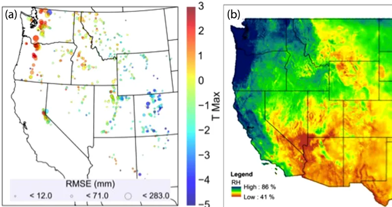
Figure 3.The optimized critical maximum daily temperature threshold that produced the lowest root mean square error (RMSE) in the prediction of snowfall at Snow Telemetry (SNOTEL) stations across the western USA (adapted from Rajagopal and Harpold, 2016). (b)Precipitation-day relative humidity averaged over 1981–2015 based on the Gridmet dataset (Abatzoglou, 2013).

the Cloud Profiling Radar (CPR) onboard CloudSat (2006 to present). The CPR operates at 94 GHz with an along-track (or vertical) resolution of ∼1.5 km. Retrieval of dry snowfall rate from CPR measurements of reflectivity have been shown to correspond with estimates of snowfall from ground-based radars at elevations of 2.6 and 3.6 km above mean sea level (Matrosov et al., 2008). Estimates at lower elevations, especially those in the lowest 1 km, are contam-inated by ground clutter. Alternative approaches, combin-ing CPR data with ancillary data have been formulated to account for this challenge (Kulie and Bennartz, 2009; Liu, 2008). Known relationships between CPR reflectivity data and the scattering properties of non-spherical ice crystals are used to derive snowfall at a given elevation above mean sea level; below this elevation a temperature threshold derived from surface data is used to discriminate between rain and snow events. Liu (2008) used 2◦_{C as the snow–rain} thresh-old, whereas Kulie and Bennartz (2009) used 0◦C as the snow–rain threshold. Temperature thresholds have been the subject of much research and debate for discriminating pre-cipitation phase, as is further discussed in Sect. 4.1.

CloudSat is part of the A-train or afternoon constella-tion of satellites, which includes Aqua, with the Moderate Resolution Imaging Spectrometer (MODIS) and the Cloud– Aerosol Lidar and Infrared Pathfinder Satellite Observations (CALIPSO) spacecraft with cloud-profiling lidar. The sen-sors onboard A-train satellites provided the unique combi-nation of data to create an operational snow retrieval prod-uct. The CPR level 2 snow profile product (2C-SNOW-PROFILE) uses vertical profile data from the CPR, input from MODIS and the CPR, as well as weather forecast data

to estimate near-surface snowfall (Kulie et al., 2016; Wood et al., 2013). The performance of 2C-SNOW-PROFILE was tested by Cao et al. (2014). This group found the product worked well in detecting light snow but performed less sat-isfactorily under conditions of moderate to heavy snow be-cause of the non-stationary effects of attenuation on the re-turned radar signal.

snow-fall is not unique. For the GPM mission, it will be neces-sary to include more variables from dual-frequency radar measurements, multiple-frequency passive microwave mea-surements, or a combination of radar and passive microwave measurement (Skofronick-Jackson et al., 2015).

4 Current tools for predicting precipitation phase 4.1 Prediction techniques from ground-based

observations

Discriminating between solid and liquid precipitation is of-ten based on a near-surface air temperature threshold (Mar-tinec and Rango, 1986; US Army Corps of Engineers, 1956; L’hôte et al., 2005). Four prediction methods have been de-veloped that use near-surface air temperature for discriminat-ing precipitation phase: (1) static threshold, (2) linear transi-tion, (3) minimum and maximum temperature, and (4) sig-moidal curve (Table 1). A static temperature threshold ap-plies a single temperature value, such as mean daily tempera-ture, where all of the precipitation above the threshold is rain, and all below the threshold is snow. Typically this threshold temperature is near 0◦C (Lynch-Stieglitz, 1994; Motoyama, 1990), but was shown to be highly variable across both space and time (Kienzle, 2008; Motoyama, 1990; Braun, 1984; Ye et al., 2013). For example, Rajagopal and Harpold (2016) op-timized a single temperature threshold at Snow Telemetry (SNOTEL) sites across the western USA to show regional variability from−4 to 3◦C (Fig. 3). A second discrimina-tion technique is to linearly scale the propordiscrimina-tion of snow and rain between a temperature for all rain (Train) and a

temper-ature for all snow (Tsnow) (Pipes and Quick, 1977; McCabe

and Wolock, 2010; Tarboton et al., 1995). Linear threshold models have been parameterized slightly differently across studies, e.g., Tsnow= −1.0 andTrain=3.0◦C (McCabe and

Wolock, 2010), Tsnow= −1.1 and Train=3.3◦C (Tarboton

et al., 1995), and Tsnow=0 andTrain=5◦C (McCabe and

Wolock, 1999b). A third technique specifies a threshold tem-perature based on daily minimum and maximum tempera-tures to classify rain and snow, respectively, with a threshold temperature between the daily minimum and maximum pro-ducing a proportion of rain and snow (Leavesley et al., 1996). This technique can have a time-varying temperature thresh-old or include aTrainthat is independent of daily maximum

temperature. A fourth technique applies a sigmoidal relation-ship between mean daily (or sub-daily) temperature and the proportion or probability of snow versus rain. For example, one method derived for southern Alberta, Canada, employs a curvilinear relationship defined by two variables, a mean daily temperature threshold where 50 % of precipitation is snow, and a temperature range where mixed-phase precipi-tation can occur (Kienzle, 2008). Another sigmoidal-based empirical model identified a hyperbolic tangent function de-fined by four parameters to estimate the conditional snow (or

rain) frequency based on a global analysis of precipitation-phase observations from over 15 000 land-based stations (Dai, 2008). Selection of temperature-based techniques is typically based on available data, with a limited number of studies quantifying their relative accuracy for hydrological applications (Harder and Pomeroy, 2014).

Several studies have compared the accuracy of temperature-based PPM to one another and/or against an independent validation of precipitation phase. Sevruk (1984) found that only about 68 % of the variability in monthly observed snow proportion in Switzerland could be explained by threshold temperature-based methods near 0◦C. An analysis of data from 15 stations in southern Alberta, Canada, with an average of > 30 years of direct observations noted overestimations in the mean annual snowfall for static threshold (8.1 %), linear transition (8.2 %), minimum and maximum (9.6 %), and sigmoidal transition-based (7.1 %) methods (Kienzle, 2008). An evaluation of PPM at three sites in the Canadian Rockies by Harder and Pomeroy (2013) found the largest percent error to occur using a static threshold (11 to 18 %), followed by linear relationships (−8 to 11 %), followed by sigmoidal relationships (−3 to 11 %). Another study using 824 stations in China with > 30 years of direct observations found accuracies of 51.4 % using a static 2.2◦C threshold and 35.7 to 47.4 % using linear temperature-based thresholds (Ding et al., 2014). Lastly, for multiple sites across the rain–snow transition in southwestern Idaho, static temperature thresholds produced the lowest proportion (68 %) of snow, whereas a linear-based model produced the highest proportion (75 %) of snow (Marks et al., 2013). These accuracy assessments generally demonstrated that static threshold methods produced the greatest errors, whereas sigmoidal relationships produced the smallest errors, although variations to this general rule existed across sites. Near-surface humidity also influences precipitation phase (see Sect. 2). Three humidity-dependent precipitation-phase identification methods are found in the literature: (1) dew point temperature (Td), (2) wet bulb

temperature (Tw), and (3) psychometric energy balance. The

dew point temperature is the temperature at which an air parcel with a fixed pressure and moisture content would be saturated. In one approach to account for measurement and instrument calibration uncertainties of ±0.25◦C, both Td

and Tw below −0.5◦C were assumed to be all snow and

above +0.5◦C all rain, with a linear relationship between the two being a proportional mix of snow and rain (Marks et al., 2013). Td of 0.0◦C performed consistently better

thanTa in one study by Marks et al. (2001) while a Td of

0.1◦C for multiple stations in Sweden was less accurate than a Ta of 1.0◦C (Feiccabrino et al., 2013). The wet or

ice bulb temperature (Tw)is the temperature at which an air

prediction (Olsen, 2003; Ding et al., 2014; Marks et al., 2013).Twsignificantly improved prediction of precipitation

phase over Ta at 15 min time steps, but only marginally

improved predictions at daily time steps (Marks et al., 2013). Ding et al. (2014) developed a sigmoidal-phase probability curve based on Tw and an elevation that outperformed Ta

threshold-based methods across a network of sites in China. Conceptually, the hydrometeor temperature (Ti) is similar

to Tw but is calculated using the latent heat and vapor

density gradient. Use of computed Ti values significantly

improved precipitation-phase estimates overTa, particularly

as timescales approached 1 day (Harder and Pomeroy, 2013). There has been limited validation of humidity-based precipitation-phase prediction techniques against ground-truth observations. Ding et al. (2014) showed that a method based onTw and elevation increased accuracy by 4.8–8.9 %

over several temperature-based methods. Their method was more accurate than the simpler Tw-based method by

Ya-mazaki (2001). Feiccabrino et al. (2013) showed thatTd

mis-classified 3.0 % of snow and rain (excluding mixed-phase precipitation), whereas Ta only misclassified 2.4 %. Ye et

al. (2013) foundTdless sensitive to phase discrimination

un-der diverse environmental conditions and seasons than Ta.

Froidurot et al. (2014) evaluated several techniques with a critical success index (CSI) at sites across Switzerland to show the highest CSI values were associated with vari-ables that includedTwor relative humidity (CSI=84–85 %)

compared to Ta (CSI=78 %). Marks et al. (2013)

evalu-ated the time at which precipitation transitioned from snow to rain against field observations across a range of eleva-tions and found that Td most closely predicted the timing

of phase change, whereas both Ta andTw estimated earlier

phase changes than observed. Harder and Pomeroy (2013) compared Ti with field observations and found that error

was < 10 % when Ti was allowed to vary with each daily

time step and > 10 % when Ti was fixed at 0◦C. The Ti

accuracy increased appreciably (i.e., 5–10 % improvement) when the temporal resolution was decreased from daily to hourly or 15 min time steps. The validation studies consis-tently showed improvements in accuracy by including hu-midity over PPMs based only on temperature.

Hydrological models employ a variety of techniques for phase prediction using ground-based observations (Ta-ble 2). All discrete hydrological models (i.e., not coupled to an atmospheric model) investigated used temperature-based thresholds that did not consider the near-surface hu-midity. Moreover, most models use a single static temper-ature threshold that typically produces lower accuracy than multiple temperature methods. It should be noted that many of these hydrological models lump by elevation zone, which improves estimates of the snow to rain transition elevation and phase prediction accuracy in complex terrain compared to models without elevation zones. Hydrological models that are coupled to atmospheric models were more able to con-sider important controls on precipitation phase, such as

hu-midity and atmospheric profiles. This compendium of model PPMs highlights the current shortcomings in phase predic-tion in convenpredic-tional discrete hydrological models.

4.2 Prediction techniques incorporating atmospheric information

param-Developing/testing/ validating phase prediction

techniques Incorporate new information into phase

prediction techniques

Atmospheric info. (reanalysis, WRF, RADAR) Near-surface humidity

(observations, reanalysis)

Improve ground-based observations of phase

Disdrometers

(NOAA, others)

Coupled observations

(SNOTEL, others)

Direct observations

(COOP stations, CoCORAHS)

Developing and testing gridded phase products

Improve hydrological modeling

Quantify and understand regional variability/

sensitivity

Communicate importance to hydrological community

Focused field campaigns

(e.g. GCPEx)

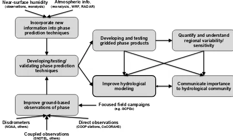
Figure 4.Conceptual representation of the research gaps and workflows needed to advance PPM and improve hydrological modeling.

eterizations lead to different spatial distributions of precipita-tion and produce varying vertical distribuprecipita-tions of hydromete-ors (Gilmore et al., 2004). Regardless, precipitation rates for each grid cell are averages requiring hydrological modelers to consider the effects of elevation, aspect, etc., in resolving precipitation-phase fractions for finer-scale models.

Numerical models that contain sophisticated cloud micro-physics schemes allow for assimilation of additional remote sensing data beyond conventional synoptic/large-scale obser-vations (balloon data). This is because the coarse spatial and temporal nature of radiosonde data results in the atmosphere being sensed imperfectly/incompletely compared with the scale of motion that weather simulation models can numer-ically resolve. These observational inadequacies are exacer-bated in complex terrain, where precipitation-phase fraction can vary on small scales and radar can be blocked by to-pography and therefore rendered useless in the model initial-ization. Accurate generation of liquid and frozen precipita-tion from vapor requires accurate depicprecipita-tion of initial atmo-spheric moisture conditions (Kalnay and Cai, 2003; Lewis et al., 2006). In acknowledgement of the difficulty and un-certainty of initializing numerical simulation models, atmo-spheric modelers use the term “bogusing” to describe incor-poration of individual observations at a point location into large-scale initial conditions in an effort to enhance the ac-curacy of the simulation (Eddington, 1989). They also

em-ploy complex assimilation methodologies to force the early period of the model solutions during the time integration to-wards fine-scale observations (Kalnay and Cai, 2003; Lewis et al., 2006). These asynoptic or fine-scale data sources often substantially improve the accuracy of the simulations as time progresses.

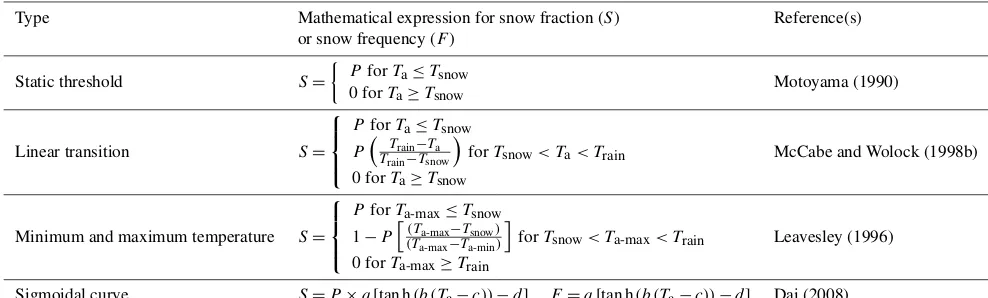
Table 1.Mathematical expression for the four common temperature-based PPM to estimate snow fraction (S) or snow frequency (F) using the mean air temperature (Ta), maximum daily air temperature (Ta-max), and/or minimum daily air temperature (Ta-min). The variableTsnow is air temperature when all precipitation (P) is snow andTrainis the air temperature when all air precipitation is rain.

Type Mathematical expression for snow fraction (S) Reference(s) or snow frequency (F)

Static threshold S=

PforTa≤Tsnow

0 forTa≥Tsnow Motoyama (1990)

Linear transition S=

  

 

P forT_a≤T_snow P Train−Ta

Train−Tsnow

forTsnow< 0 forTa≥Tsnow

Ta< Train McCabe and Wolock (1998b)

Minimum and maximum temperature S=   

 

P forT_a-max≤T_snow 1−Ph(Ta-max−Tsnow) (Ta-max−Ta-min) i

forTsnow< Ta-max< Train 0 forTa-max≥Train

Leavesley (1996)

Sigmoidal curve S=P×a[tan h(b (Ta−c))−d] F=a[tan h(b (Ta−c))−d] Dai (2008)

5 Research gaps

The incorrect prediction of precipitation phase leads to cas-cading effects on hydrological simulations (Fig. 1). Meeting the challenge of accurately predicting precipitation phase re-quires the closing of several critical research gaps (Fig. 4). Perhaps the most pressing challenge for improving PPMs is developing and employing new and improved sources of data. However, new data sources will not yield much ben-efit without effective incorporation into predictive models (Fig. 4). Additionally, both the scientific and management communities lack data products that can be readily under-stood and broadly used. Addressing these research gaps re-quires simultaneous engagement both within and between the hydrology and atmospheric observation and modeling communities. Changes to atmospheric temperature and hu-midity profiles from regional climate change will likely chal-lenge conventional precipitation-phase prediction in ways that demand additional observations and improved forecasts. We also highlight research gaps to improve relatively sim-ple hydrological models without adding unnecessary com-plexity associated with sophisticated PPM approaches. For example, more efforts to verify the existing PPMs in different climatic environments and during specific hydrometeorolog-ical events could help determine various temperature thresh-olds (Table 1) to apply in of the existing models (Sect. 5.3). In addition, developing gridded precipitation-phase products may eliminate the need to make existing models more com-plex by applying more comcom-plex PPMs outside of those mod-els, e.g., similar to precipitation distribution in existing grid-ded products used by many hydrological models. Ultimately, recognizing the sensitivity of hydrological model outcomes to PPMs and identifying which climates and applications re-quire higher-phase prediction accuracy are crucial steps to determining the complexity of PPMs required for specific ap-plications.

5.1 Conduct focused field campaigns

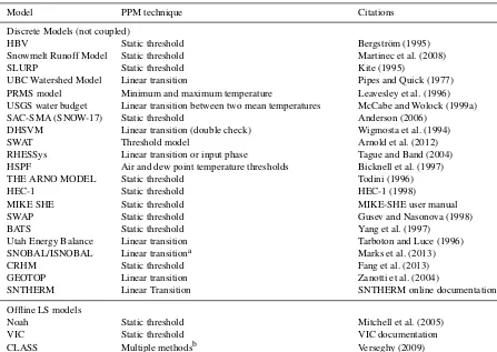
Table 2.Common hydrological models and the phase partitioning method (PPM) technique employed. The citation referring to the original publication of the model is given.

Model PPM technique Citations

Discrete Models (not coupled)

HBV Static threshold Bergström (1995)

Snowmelt Runoff Model Static threshold Martinec et al. (2008)

SLURP Static threshold Kite (1995)

UBC Watershed Model Linear transition Pipes and Quick (1977)

PRMS model Minimum and maximum temperature Leavesley et al. (1996)

USGS water budget Linear transition between two mean temperatures McCabe and Wolock (1999a)

SAC-SMA (SNOW-17) Static threshold Anderson (2006)

DHSVM Linear transition (double check) Wigmosta et al. (1994)

SWAT Threshold model Arnold et al. (2012)

RHESSys Linear transition or input phase Tague and Band (2004)

HSPF Air and dew point temperature thresholds Bicknell et al. (1997)

THE ARNO MODEL Static threshold Todini (1996)

HEC-1 Static threshold HEC-1 (1998)

MIKE SHE Static threshold MIKE-SHE user manual

SWAP Static threshold Gusev and Nasonova (1998)

BATS Static threshold Yang et al. (1997)

Utah Energy Balance Linear transition Tarboton and Luce (1996)

SNOBAL/ISNOBAL Linear transitiona Marks et al. (2013)

CRHM Static threshold Fang et al. (2013)

GEOTOP Linear transition Zanotti et al. (2004)

SNTHERM Linear Transition SNTHERM online documentation

Offline LS models

Noah Static threshold Mitchell et al. (2005)

VIC Static threshold VIC documentation

CLASS Multiple methodsb Verseghy (2009)

a_{By default. Temperature-phase–density relationship explicitly specified by user.}b_{A flag is specified, which switches between static threshold and linear} transition.

5.2 Incorporate humidity information

Atmospheric humidity affects the energy budget of falling hydrometeors (Sect. 4.1), but is rarely considered in precipitation-phase prediction. The difficulty in incorporat-ing humidity mainly arises from a lack of observations, both as point measurements and distributed gridded products. For example, while some reanalysis products have humidity in-formation (i.e., National Centers for Environmental Predic-tion, NCEP reanalysis) they are at spatial scales (i.e., > 1◦) that are too coarse for resolving precipitation phase in com-plex topography. Addition of high-quality aspirated humidity sensors at snow-monitoring stations, such as the SNOTEL network, would advance our understanding of humidity and its effects on precipitation phase in the mountains. Because dry air masses have regional variations controlled by storm tracks and proximity to water bodies, sensitivity of precipita-tion phase to humidity variaprecipita-tions driven by regional warming remains relatively unexplored.

Although humidity datasets are relatively rare in mountain environments, some gridded data products exist that can be used to investigate the importance of humidity information.

Most interpolated gridded data products either do not include any measure of humidity (e.g., Daymet or WorldClim) or use daily temperature measurements to infer humidity conditions (e.g., PRISM). In complex terrain, air temperature can also vary dramatically at relatively small scales from ridge tops to valley bottoms due to cold air drainage (Whiteman et al., 1999) and hence can introduce errors into inferential tech-niques such as these. Potentially more useful are data assim-ilation products, such as NLDAS-2, that provide humidity and temperature values at 1/8th of a degree scale over the continental USA. In addition, several data reanalysis prod-ucts are often available at 1–3-year lags from present, in-cluding NCEP/NCAR, NARR, and the 20th century reanaly-sis. Given the relatively sparse observations of humidity in mountain environments, the accuracy of gridded humidity products is rarely rigorously evaluated (Abatzoglou, 2013). More work is needed to understand the added skill provided by humidity datasets for predicting precipitation phase and its distribution over time and space.

tion and additional verification of the skill in phase prediction provided by atmospheric information.

Several avenues exist to better incorporate atmospheric in-formation into precipitation-phase prediction, including di-rect observations, remote sensing observations, and synthetic products. Radiosonde measurements made daily at many airports and weather forecasting centers have shown some promise for supplying atmospheric profiles of temperature and humidity (Froidurot et al., 2014). However, these data are only useful to initialize the larger-scale structure of tem-perature and water vapor, and may not capture local-scale variations in complex terrain. It is also their lack of tem-poral and spatial frequency that prevents their use in ac-curate precipitation-phase prediction, which is inherently a mesoscale problem, i.e., scales of motion < 100 km. Atmo-spheric information on the bright-band height from Doppler radar has been utilized for predicting the altitude of the rain–snow transition (Lundquist et al., 2008; Minder, 2010), but has rarely been incorporated into hydrological model-ing applications (Maurer and Mass, 2006; Mizukami et al., 2013). In addition to atmospheric observations, modeling products that assimilate observations or are fully physically based may provide additional information for precipitation-phase prediction. Numerous reanalysis products (described in Sect. 2.2) provide temperature and humidity at different pressure levels within the atmosphere. To our knowledge, in-formation from reanalysis products has yet to be incorpo-rated into precipitation-phase prediction for hydrological ap-plications. Bulk microphysical schemes used by meteorolog-ical models (e.g., WRF) provide physmeteorolog-ically based estimates of precipitation phase. These schemes capture a wide vari-ety of processes, including evaporation, sublimation, con-densation, and aggradation, and output between two and ten precipitation types. Historically, meteorological models have not been run at spatial scales capable of resolving con-vective dynamics (e.g., < 2 km), which can exacerbate er-ror in precipitation-phase prediction in complex terrain with a moist neutral atmosphere. Coarse meteorological models also struggle to produce pockets of frozen precipitation from advection of moisture plumes between mountain ranges and cold air wedged between topographic barriers. However, re-duced computational restrictions on running these models at finer spatial scales and over large geographic extents (Ras-mussen et al., 2012) are enabling further investigations into precipitation-phase change under historical and future cli-mate scenarios. This suggests that finer dynamical downscal-ing is necessary to resolve precipitation phase, which is con-sistent with similar work attempting to resolve winter precip-itation amounts in complex terrain (Gutmann et al., 2012). A potentially impactful area of research is to integrate this information into novel approaches to improve precipitation-phase prediction skill.

5.3 Disdrometer networks operating at high temporal resolutions

An increase in the types and reliability of disdrometers over the last decade has provided a new suite of tools to more di-rectly measure precipitation phase. Despite this new poten-tial resource for distinguishing snow and rain, very limited deployments of disdrometers have occurred at the scale nec-essary to improve hydrologic modeling and rain–snow ele-vation estimates. The lack of disdrometer deployment likely arises from a number of potential limitations: (1) known is-sues with accuracy, (2) cost of these systems, and (3) power requirements needed for heating elements. These limitations are clearly a factor in procuring large networks and deploy-ing disdrometers in complex terrain that is remote and fre-quently difficult to access. However, we advise that disdrom-eters offer numerous benefits that cannot be substituted with other measurements: (1) they operate at fine temporal scales, (2) they operate in low-light conditions that limit other direct observations, and (3) they provide land surface observations rather than precipitation phase in the atmosphere (as com-pared to more remote methods). Moreover, improvements in disdrometer and power supply technologies that address these limitations would remove restrictions on increased dis-drometer deployment.

Transects of disdrometers spanning the rain–snow eleva-tions of key mountain areas could add substantially to both prediction of precipitation phase for modeling purposes, as well as validating typical predictive models. We advocate for transects over key mountain passes where power is gener-ally available and weather forecasts for travel are particu-larly important. In addition, co-locating disdrometers at long-term research stations, where precipitation-phase observa-tions could be tied to micro-meteorological and hydrological observations, has distinct advantages. These areas often have power supplies and instrumentation expertise to operate and maintain disdrometer networks.

5.4 Compare different indirect-phase measurement methods

condi-tions. Similarly, employing coupled observations of precip-itation and snow depth has been used to assess accuracy of different precipitation phase prediction methods (Marks et al., 2013; Harder and Pomeroy, 2013), but accuracy assess-ment of these techniques themselves are lacking under a wide range of contrasting hydrometeorological conditions.

A variety of accuracy assessments are needed that will require co-located distributed measurements. One critical accuracy assessment involves the consistency of different precipitation-phase prediction methods under different cli-mate and atmospheric conditions. Assessing the effects of climate and atmospheric conditions requires measurements from a variety of sites covering a range of hydroclimatic con-ditions and record lengths that span the conceivable range of atmospheric conditions at a given site. Another impor-tant evaluation metric is the performance over different time steps. Harder and Pomeroy (2013) showed that hydrometeor and temperature-based prediction methods had errors that substantially decreased across shorter time steps. Identify-ing the effects of time step length on the accuracy of differ-ent prediction methods has been relatively unexplored, but is critical to select the most appropriate method for specific hydrological applications. Finally, the performance metrics used to assess accuracy should be carefully considered. The applications of precipitation phase prediction methods are di-verse, necessitating a wide variety of performance metrics, including the probability of snow versus rain (Dai, 2008), the error in annual or total snow/rain accumulation (Rajagopal and Harpold, 2016), performance under extreme conditions of precipitation amount and intensity, determination of the snow–rain elevation (Marks et al., 2013), and uncertainty arising from measurement error and accuracy. Comparison of different metrics across a wide variety of sites and condi-tions is lacking but is greatly needed to advance hydrologic science in cold regions.

5.5 Develop spatially resolved products

Many hydrological applications will benefit from gridded data products that are easily integrated into standard hydro-logical models. Currently, very few options exist for gridded data precipitation-phase products. Instead, most hydrological models have some type of submodel or simple scheme that specifies precipitation phase as rain, snow, or mixed-phase precipitation (see Sect. 4). While testing PPMs with ground-based observations could lead to improved submodels, we believe development of gridded forcing data may be an easier and more effective solution for many hydrological modeling applications.

Gridded data products could be derived from a combina-tion of remote sensing and existing synthetic products, but would need to be extensively evaluated. The NASA GPM mission is beginning to produce gridded precipitation-phase products at 3 h and 0.1◦resolution. However, GPM phase is measured at the top of the atmosphere, typically relies on

simple temperature thresholds, and has yet to be validated with ground-based observations. Another existing product is the Snow Data Assimilation System (SNODAS) that esti-mates liquid and solid precipitation at the 1 km scale. How-ever, the developers of SNODAS caution that it is not suit-able for estimating storm totals or regional differences. Fur-thermore, to our knowledge the precipitation-phase product from SNODAS has not been validated with ground observa-tions. We suggest the development of new gridded data prod-ucts that utilize new PPMs (i.e., Harder and Pomeroy, 2013) and new and expanded observational datasets, such as atmo-spheric information and radar estimates. We advocate for the development of multiple gridded products that can be evalu-ated with surface observations to compare and contrast their strengths. Accurate gridded-phase products rely on the abil-ity to represent the physics of water vapor and energy flows in complex terrain (e.g., Holden et al., 2010), where statisti-cal downsstatisti-caling methods are typistatisti-cally insufficient (Gutmann et al., 2012). This would also allow for ensembles of phase estimates to be used in hydrological models, similar to what is currently being done with gridded precipitation estimates.

5.6 Characterization of regional variability and response to climate change

of the main challenges in using remotely sensed data for dis-tinguishing between frozen and liquid hydrometeors is the lack of validation. Where products have been validated, the results are usually only relevant for the locale of the study area. Spaceborne radar combined with ground-based radar offers perhaps the most promising solution, but given the non-unique relationship between radar reflectivity and snow-fall, further testing is necessary in order to develop reliable algorithms.

Future work is needed to improve projections of changes in snowpack and water availability from regional to global scales. This local to sub-regional characterization is needed for water resource prediction and to better inform decision and policy makers. In particular, the ability to predict the transitional rain–snow elevations and its uncertainty is crit-ical for a variety of end users, including state and municipal water agencies, flood forecasters, agricultural water boards, transportation agencies, and wildlife, forest, and land man-agers. Fundamental advancements in characterizing regional variability are possible by addressing the research challenges detailed in Sect. 5.1–5.5.

6 Conclusions

This review paper is a step towards communicating the po-tential bottlenecks in hydrological modeling caused by poor representation of precipitation phase (Fig. 1). Our goals are to demonstrate that major research gaps in our ability to de-velop PPMs are contributing to errors and reducing the pdictive skill of hydrological models. By highlighting the re-search gaps that could advance the science of PPMs, we pro-vide a road map for future advances (Fig. 4). While many of the research gaps are recognized by the community and are being pursued, including incorporating atmospheric and humidity information, others remain essentially unexplored (e.g., production of gridded data, widespread ground valida-tion, and remote sensing validation).

The key points that must be communicated to the hy-drologic community and its funding agencies can be dis-tilled into the following two statements: (1) current PPMs are too simple to capture important processes and are not well validated for most locations, (2) the lack of sophisti-cated PPMs increases the uncertainty in estimation of hy-drological sensitivity to changes in precipitation phase at lo-cal to regional slo-cales. We advocate for better incorporation of new information (Sect. 5.1–5.2) and improved validation methods (Sect. 5.3–5.4) to advance our current PPMs and observations. These improved PPMs and remote sensing ob-servations will be capable of developing gridded datasets (Sect. 5.5) and providing new insight that reduces the un-certainty of predicting regional changes from snow to rain (Sect. 5.6). Improved PPMs and existing phase products will also facilitate improvement of simpler hydrological models for which more complex PPMs are not justified. A concerted

effort by the hydrological and atmospheric science commu-nities to address the PPM challenge will remedy current lim-itations in hydrological modeling of precipitation phase, ad-vance the understanding of cold regions hydrology, and pro-vide better information to decision makers.

7 Data availability

Datasets used to create Fig. 3 are available for the SNO-TEL site at the following link: https://wcc.sc.egov.usda.gov/ reportGenerator/ (last access: 19 December 2016) and for the University of Idaho Gridded Surface Meteorological Data at the following link: https://www.northwestknowledge.net/ metdata/data/ (last access: 19 December 2016).

Acknowledgements. This work was conducted as a part of an Innovation Working Group supported by the Idaho, Nevada, and New Mexico EPSCoR Programs and by the National Science Foundation under award numbers IIA-1329469, IIA-1329470, and IIA-1329513. Adrian Harpold was partially supported by USDA NIFA NEV05293. Adrian Harpold and Rina Schumer were supported by the NASA EPSCOR cooperative agreement no. NNX14AN24A. Timothy Link was partially supported by the Department of the Interior Northwest Climate Science Center (NW CSC) through a cooperative agreement no. G14AP00153 from the United States Geological Survey (USGS). Seshadri Rajagopal was partially supported by research supported by NSF/USDA grant (nos. 1360506 and 1360507) and startup funds provided by Desert Research Institute. The contents of this manuscript are solely the findings/opinions of the authors and do not necessarily represent the views of the NW CSC or the USGS. This manuscript is submitted for publication with the understanding that the United States Government is authorized to reproduce and distribute reprints for Governmental purposes.

Edited by: J. Seibert

Reviewed by: two anonymous referees

References

Abatzoglou, J. T.: Development of gridded surface meteorological data for ecological applications and modelling, Int. J. Climatol., 33, 121–131, doi:10.1002/joc.3413, 2013.

Anderson, E.: Snow Accumulation and Ablation Model – Snow-17, available at: http://www.nws.noaa.gov/oh/hrl/nwsrfs/users_ manual/part2/_pdf/22snow17.pdf, (last access: 22 August 2016), 2006,

Arkin, P. A. and Ardanuy, P. E.: Estimating climatic-scale precipi-tation from space: a review, J. Climate, 2, 1229–1238, 1989. Arnold, J. G., Kiniry, J. R., Srinivasan R., Williams, J. R, Haney, E.

B., and Neitsch S. L.: SWAT Input/Output Documentation, Texas Water Resources Institute, TR-439, available at: http://swat. tamu.edu/media/69296/SWAT-IO-Documentation-2012.pdf, (last access: 22 August 2016), 2012,

western United States, Water Resour. Res., 42, W08432, doi:10.1029/2005wr004387, 2006.

Barnett, T. P., Adam, J. C., and Lettenmaier, D. P.: Potential impacts of a warming climate on water availability in snow-dominated regions, Nature, 438, 303–309, doi:10.1038/nature04141, 2005. Battaglia, A., Rustemeier, E., Tokay, A., Blahak, U., and

Simmer, C.: PARSIVEL Snow Observations: A Crit-ical Assessment, J. Atmos. Ocean. Tech., 27, 333–344, doi:10.1175/2009jtecha1332.1, 2010.

Berghuijs, W. R., Woods, R. A., and Hrachowitz, M.: A pre-cipitation shift from snow towards rain leads to a de-crease in streamflow, Nature Climate Change, 4, 583–586, doi:10.1038/nclimate2246, 2014.

Bergström, S.: The HBV model, in: Computer Models of Watershed Hydrology, edited by: Singh, V. P., Water Resour. Publications, Highlands Ranch, CO, 443–476, 1995.

Bernauer, F., Hurkamp, K., Ruhm, W., and Tschiersch, J.: Snow event classification with a 2D video disdrometer – A decision tree approach, Atmos. Res., 172, 186–195, 2016.

Berris, S. N. and Harr, R. D.: Comparative snow accumulation and melt during rainfall in forested and clear-cut plots in the Western Cascades of Oregon, Water Resour. Res., 23, 135–142, doi:10.1029/WR023i001p00135, 1987.

Bicknell, B. R., Imhoff, J. C., Kittle Jr., J. L., Donigian Jr., A. S., and Johanson, R. C.: Hydrological Simulation Program–Fortran, User’s manual for version 11: US Environmental Protection Agency, National Exposure Research Laboratory, Athens, Ga., EPA/600/R-97/080, p. 755, 1997.

Boe, E. T.: Assessing Local Snow Variability Using a Network of Ultrasonic Snow Depth Sensors, Master of Science in Hydro-logic Sciences, Geosciences, Boise State, 2013.

Boodoo, S., Hudak, D., Donaldson, N., and Leduc, M.: Ap-plication of Dual-Polarization Radar Melting-Layer Detec-tion Algorithm, J. Appl. Meteorol. Climatol., 49, 1779–1793, doi:10.1175/2010jamc2421.1, 2010.

Borrmann, S. and Jaenicke, R.: Application of microholography for ground-based in-situ measurements in stratus cloud layers – a case study, J. Atmos. Ocean. Tech., 10, 277–293, 1993. Braun, L. N.: Simulation of snowmelt-runoff in lowland and lower

alpine regions of Switzerland, Diss. Naturwiss, ETH Zürich, Nr. 7684 0000, edited by: Ohmura, A., Vischer, D., and Lang, H., 1984.

Cao, Q., Hong, Y., Chen, S., Gourley, J. J., Zhang, J., and Kirstet-ter, P. E.: Snowfall Detectability of NASA’s CloudSat: The First Cross-Investigation of Its 2C-Snow-Profile Product and National Multi-Sensor Mosaic QPE (NMQ) Snowfall Data, Prog. Electro-magn. Res., 148, 55–61, doi:10.2528/pier14030405, 2014. Cayan, D. R., Kammerdiener, S. A., Dettinger, M. D., Caprio, J. M.,

and Peterson, D. H.: Changes in the onset of spring in the western United States, B. Am. Meteorol. Soc., 82, 399–415, 2001. Chandrasekar, V., Keranen, R., Lim, S., and Moisseev, D.:

Re-cent advances in classification of observations from dual polarization weather radars, Atmos. Res., 119, 97–111, doi:10.1016/j.atmosres.2011.08.014, 2013.

Chen, S., Gourley, J. J., Hong, Y., Cao, Q., Carr, N., Kirstetter, P.-E., Zhang, J., and Flamig, Z.: Using citizen science reports to eval-uate estimates of surface precipitation type, B. Am. Meteorol. Soc., 187–193, doi:10.1175/BAMS-D-13-00247.1, 2015.

Dai, A.: Temperature and pressure dependence of the rain-snow phase transition over land and ocean, Geophys. Res. Lett., 35, L12802, doi:10.1029/2008gl033295, 2008.

Ding, B., Yang, K., Qin, J., Wang, L., Chen, Y., and He, X.: The dependence of precipitation types on surface elevation and me-teorological conditions and its parameterization, J. Hydrol., 513, 154–163, doi:10.1016/j.jhydrol.2014.03.038, 2014.

Eddington, L. W.: Satellite-Derived Moisture-Bogusing Profiles for the North Atlantic Ocean, DTIC Document, 1989.

Elmore, K. L.: The NSSL Hydrometeor Classification Algorithm in Winter Surface Precipitation: Evaluation and Future Devel-opment, Weather Forecast., 26, 756–765, doi:10.1175/waf-d-10-05011.1, 2011.

Fang, X., Pomeroy, J. W., Ellis, C. R., MacDonald, M. K., De-Beer, C. M., and Brown, T.: Multi-variable evaluation of hy-drological model predictions for a headwater basin in the Cana-dian Rocky Mountains, Hydrol. Earth Syst. Sci., 17, 1635–1659, doi:10.5194/hess-17-1635-2013, 2013.

Fatichi, S., Vivoni, E. R., Ogden, F. L., Ivanov, V. Y., Mirus, B., Gochis, D., Downer, C. W., Camporese, M., Davison, J. H., Ebel, B., Jones, N., Kim, J., Mascaro, G., Niswonger, R., Re-strepo, P., Rigon, R., Shen, C., Sulis, M., and Tarboton, D.: An overview of current applications, challenges, and future trends in distributed process-based models in hydrology, J. Hydrol., 537, 45–60, 2016.

Feiccabrino, J., Lundberg, A., and Gustafsson, D.: Improving surface-based precipitation phase determination through air mass boundary identification, Hydrol. Rese., 43, 179–191, doi:10.2166/nh.2012.060, 2013.

Feiccabrino, J., Gustafsson, D., and Lundberg, A.: Surface-based precipitation phase determination methods in hydrological mod-els, Hydrol. Res., 44, 44–57, 2015.

Floyd, W. and Weiler, M.: Measuring snow accumulation and ablation dynamics during rain-on-snow events: innova-tive measurement techniques, Hydrol. Proc., 22, 4805–4812, doi:10.1002/hyp.7142, 2008.

Fritze, H., Stewart, I. T., and Pebesma, E.: Shifts in West-ern North American Snowmelt Runoff Regimes for the Recent Warm Decades, J. Hydrometeorol., 12, 989–1006, doi:10.1175/2011jhm1360.1, 2011.

Froidurot, S., Zin, I., Hingray, B., and Gautheron, A.: Sensi-tivity of Precipitation Phase over the Swiss Alps to Differ-ent Meteorological Variables, J. Hydrometeorol., 15, 685–696, doi:10.1175/jhm-d-13-073.1, 2014.

Garvelmann, J., Pohl, S., and Weiler, M.: From observation to the quantification of snow processes with a time-lapse camera network, Hydrol. Earth Syst. Sci., 17, 1415–1429, doi:10.5194/hess-17-1415-2013, 2013.

Giangrande, S. E., Krause, J. M., and Ryzhkov, A. V.: Automatic designation of the melting layer with a polarimetric prototype of the WSR-88D radar, J. Appl. Meteorol. Climatol., 47, 1354– 1364, doi:10.1175/2007jamc1634.1, 2008.

Gilmore, M. S., Straka, J. M., and Rasmussen, E. N.: Precipitation Uncertainty Due to Variations in Precipitation Particle Parame-ters within a Simple Microphysics Scheme, Mon. Weather Rev., 132, 2610–2627, doi:10.1175/MWR2810.1, 2004.