Evaluation of artificial neural network techniques for flow
forecasting in the River Yangtze, China
C.W. Dawson
1,
C. Harpham
2,
R.L. Wilby
3and
Y. Chen
41Department of Computer Science, Loughborough University, Leicestershire, LE11 3TU, UK
2School of Computing and Technology, University of Derby, Kedleston Road, Derby, DE22 1GB, UK
3Department of Geography, King’s College London, Strand, London, WC2R 2LS, UK
4Institute of Hydrology and Water Resources, Three Gorges University, Yichang, Hubei, China
Email for corresponding author: [email protected]
Abstract
While engineers have been quantifying rainfall-runoff processes since the mid-19th century, it is only in the last decade that artificial neural network models have been applied to the same task. This paper evaluates two neural networks in this context: the popular multilayer perceptron (MLP), and the radial basis function network (RBF). Using six-hourly rainfall-runoff data for the River Yangtze at Yichang (upstream of the Three Gorges Dam) for the period 1991 to 1993, it is shown that both neural network types can simulate river flows beyond the range of the training set. In addition, an evaluation of alternative RBF transfer functions demonstrates that the popular Gaussian function, often used in RBF networks, is not necessarily the ‘best’ function to use for river flow forecasting.Comparisons are also made between these neural networks and conventional statistical techniques; stepwise multiple linear regression, auto regressive moving average models and a zero order forecasting approach.
Keywords: Artificial neural network, multilayer perception, radial basis function, flood forecasting
Introduction
OVERVIEW
The Three Gorges Project is the world’s largest hydroelectric project. It is costing the Chinese government approximately £7.6 billion to construct a dam 2.2km long and 175m high across the River Yangtze in the Three Gorges Region, China (Chinese Embassy, 1997a) — see Fig. 1. Construction began in 1993, and the plant will start producing electricity in 2003, with full project completion in 2009. The impoundment will create a reservoir approximately 663km long and submerge 632 square km, 1599 industrial and mining enterprises and 365 townships – displacing an estimated 1.2 million people in the process (Chinese Embassy, 1997b). However, the dam will provide one seventh of China’s electrical output (compared to output in 1992) (ibid) and much needed flood control for this vast river.
This paper presents results from the development of experimental neural networks that were trained to model the flow in this region (the catchment area of which is 56,000km2). Two neural network models were used in this
China
Three Gorges Region
River Yangtze
Fig.1. Location of the Three Gorges Region in China
networks were evaluated. Thirdly, the more general problem of assigning confidence intervals to ANN model forecasts has been considered.
ARTIFICIAL NEURAL NETWORKS
Artificial neural networks are powerful tools for relating sets of predictor variables (in this case, for example, antecedent rainfall and river flows), in non-linear ways, to specified forecast variables (e.g. future river flows). Although ANNs have existed in various forms for over fifty years (McCulloch and Pitts, 1943) it is only since the rediscovery and popularisation of the backpropagation training algorithm that it has been possible to construct neural networks of any practical size and complexity (Rumelhart and McClelland, 1986). Since the 1980s, research in artificial neural networks has accelerated and today neural networks are utilized in many different applications using different network types, training algorithms and structures.
In this study, two of the most popular neural networks are examined: the widely used MLP and the less favoured RBF network. Although the MLP can produce accurate flow forecasts, it does have a number of drawbacks. For example, training an appropriate network can take a long time and a number of parameters must be determined by the neural network developer. On the other hand, although the RBF has been used in a limited number of studies (Mason et al., 1996; Jayawardena and Fernando, 1998; Dawson et al., 2000), it can be trained in a fraction of the time, has fewer parameters to be determined and, in certain cases, predicts river flow more accurately than the MLP (Jayawardena et al., 1997).
A detailed explanation of the plethora of network types and training algorithms is beyond the scope of this paper. Interested readers should refer to texts such as Bishop (1995) and Haykin (1999) for a detailed discussion on neural networks, or Maier and Dandy (2000) and Dawson and Wilby (2001) for overviews of ANN applications within hydrology (neurohydrology). Neurohydrology (a term coined by Abrahart et al., 1998) is an emerging field that draws together the expertise of the computer scientist (neural network developer) and the hydrologist. It can be described as the application of artificial neural networks to the problem of rainfall-runoff modelling and flood forecasting.
Artificial neural networks were chosen as the applied method for the present investigation for various reasons. They do not presuppose a detailed understanding of a river’s physical characteristics, nor do they require extensive data pre-processing. This is because ANNs can, theoretically, handle incomplete, noisy and ambiguous data. Furthermore,
artificial neural networks are often cheaper and simpler to implement than physically-based hydrological models. ANNs are also well suited to dynamic problems and are parsimonious in terms of information storage within the trained model.
Experiments
METHODOLOGY
For these experiments, the protocol of Dawson and Wilby (2001) was applied to rainfall-runoff data for the River Yangtze. This protocol consists of seven stages that can be summarised as:
(1) Gather data;
(2) Select predictand - what is the model trying to predict and what is to be optimised?
(3) Data preprocessing stage 1 (cleansing and identifying appropriate predictors);
(4) ANN selection - select an appropriate network type and training algorithm;
(5) Data preprocessing stage 2 (standardise the data and split into appropriate training, test and validation sets); (6) Network training - train the network(s) with the
processed data sets;
(7) Evaluation - using appropriate error measures to interpret the results.
(1) Rainfall-runoff data were obtained at six-hourly intervals for the River Yangtze, and included five flood events between early June to mid-August during 1991 to 1993 (yielding approximately 400 data points for ANN model calibration and testing). The data included discharge at two sites upstream of the Three Gorges dam site (as well as the dam site itself) and precipitation in four upstream sub-basins.
(2) Predictand — the models were trained to predict flow at six hourly intervals at the Three Gorges dam site.
(3) Due to the size and characteristics of the data set, no cleansing of the data was required at this stage. The data were analysed (using correlation and partial correlation functions) to determine the strongest relationships between discharge and previous events starting with a minimum 48 hour lead time. A minimum lead time of 48 hours was chosen as an initial point for the analyses as any shorter period would limit the effectiveness of a flood forecasting model in providing adequate warnings.
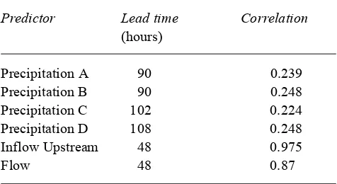
dam site (with a lead time of 48 hours). The correlations between each of these predictors and flow are presented in Table 1 along with the chosen lead times. Thus, the models were trained with six inputs and one output.
From an inspection of Table 1, it would appear that precipitation has little correlation with flow when compared with the two antecedent flow predictors. However, experimental models that excluded these parameters provided less accurate forecasts than models which included them (for example, the best MLP developed without these predictors had a RMSE of 2984 cumecs compared with 2068 cumecs when they were included). These results emphasise the importance of including all appropriate information in model calibration.
It is important to have an understanding of catchment characteristics and the hydrological processes involved before ‘blindly’ applying neural networks to the available data. The authors hope to provide a protocol for a more rigorous application of alternative models to the physical process. In the absence of such a protocol, this paper follows recognised procedures in developing the neural network models in this study. Recent work by Abrahart et al. (2001) has highlighted the ability of neural networks to infer physical processes within the rainfall-runoff cycle. This work is still ongoing and aims to provide a hydrological explanation of neural network rainfall-runoff model behaviour.
(4) Both MLP and RBF networks were used in this study. In the majority of hydrological studies with RBF networks (Dawson and Wilby, 2001), the Gaussian function is used as the transfer function. However, as the results presented later indicate, the optimal performance may not necessarily be obtained with the Gaussian function and it is advisable to try alternatives. To evaluate the effectiveness of alternative transfer functions within the RBF network, six transfer functions (ϕ(x)) were used in this study; the Gaussian (1), multiquadratic (MQ) (2), inverse multiquadratic (IMQ) (3)
(Hardy, 1971), cubic (4), linear (5) and thin plate spline (TPS) (6) (σ is the width of the transfer function):
φ
(
x
)=
exp(-2v2x2
)
for σ > 0 and x ∈ℜ (1)φ
(
x
)=
x
2+ v
2for σ > 0 and x∈ℜ (2)φ(x)=
x2+ v2
1 for
σ > 0 and x∈ℜ (3)
ϕ(x) = x3 (4)
ϕ(x) = x (5)
ϕ(x) = x2 ln(x) (6)
(5) One criticism levelled at neurohydrological models is their inability to predict values outside the range of their training data (see Minns and Hall, 1996). These events may occur because of extreme weather conditions or changing catchment characteristics. As neural networks behave as black boxes, it is difficult to incorporate catchment changes without retraining. To overcome the problem of extreme events, neural network developers often standardise data in training sets to the range [0.1, 0.9] (or similar). This attempts to accommodate test and validation events in excess of data in the training set in the boundaries [0, 0.1] and [0.9, 1]. This was the procedure adopted in this study. It is also important to standardise data to this kind of range because of the asymptotic nature of the transfer (squashing) function used in a neural network’s nodes. Values beyond these limits tend to retard training as the gradient of the transfer function approximates to zero. This leads to minute changes being made by the backpropagation algorithm to a network’s interconnecting weights during training.
The data were then split into four flood events for training (50% of the data), one flood event from 1993 for testing (10% of the data), and one flood validation event from 1992 (40% of the data). The peak flow in the training set was 49 200 cumecs while the peak flow in the validation event was 50 300 cumecs.
[image:3.595.316.552.114.293.2](6) The MLP networks were trained using the popular backpropagation algorithm from 100 to 5000 epochs with a sigmoid transfer function throughout. After every 100 epochs the models were assessed against the test set. A trial and error approach was used to select an appropriate number of nodes in each MLP’s single hidden layer, assessing 5, 10, 20 and 30 hidden nodes. In these experiments, the backpropagation learning parameter was set to 0.1 and the Table 1. Correlation between observed flows and selected
predictors (calibration data)
Predictor Lead time Correlation
(hours)
Precipitation A 90 0.239
Precipitation B 90 0.248
Precipitation C 102 0.224
Precipitation D 108 0.248
Inflow Upstream 48 0.975
Flow 48 0.87
σ
σ
momentum rate to 0.9 (values that have proved favourable in the past; see Dawson and Wilby, 1998).
The cluster centres for the RBF network were determined using K-Means clustering which involves sorting all objects into a defined number of groups by minimising the total squared Euclidean distance for each object with respect to its nearest cluster centre. Because of the speed in training the RBF network, between 2 and 50 clusters were assessed for each of the transfer functions identified above, and the most accurate model was chosen based on comparisons with the test data set.
(7) Evaluation
To compare the models with more conventional techniques parallel experiments were performed with the same data sets. These experiments resulted in the development of an ARMA model, a SWMLR (step-wise linear regression) model and ZOF (zero order forecast) model. The SWMLR adds variables to the model depending on their partial F-ratio. Variables are added into (or removed from) the model until no significant improvement in the model’s accuracy is achieved. The ARMA model uses both previous errors (shocks) of a model’s output and previous outputs from the model to predict flow. Analyses of autocorrelation, partial autocorrelation and shocks indicated no moving average term was required for the ARMA model. Thus, a multivariate AR(1) model was produced (i.e. a first order AR model with multiple input parameters). The SWMLR model retained only two of the predictors listed in Table 1; the discharge upstream and at the dam site, 48 hours prior to the forecast flow. The ZOF model used the previous 48 hours observed flow as the naïve forecast of flow.
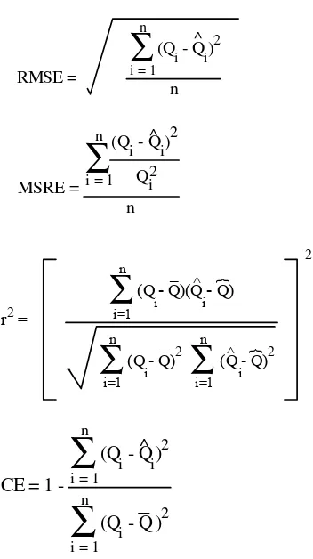
Error measures
It is important to apply multiple error measures when assessing hydrological model skill (Dawson and Wilby, 2001). Some measures provide useful insights into a model’s behaviour at high flows (e.g. root mean squared error; RMSE), others at low flows (e.g. mean squared relative error; MSRE), others can provide useful indications of a model’s overall performance (for example, R-squared), while others penalise models that have excessive numbers of parameters (e.g. A information criteria; AIC and B information criteria; BIC). In addition, it is informative to present several performance measures to allow comparisons with other studies (there being no universally accepted measure of ANN skill).
With these points in mind, the following error measures were applied (further discussion of which can be found in Legates and McCabe, 1999; Dawson and Wilby, 2001; Hall, 2001):
MSE =
n
∑
i = 1 n
(Qi - Q^i)2
R
^
MSRE = n
∑
i = 1n
Qi (Q
i - Qi) 2
2
r2 =
∑
i=1n (Q - Q)2∑
i=1 n
(Q - Q)2
∑
i=1 n
(Q - Q)(Q - Q)
2
i
_ ^
i i
i
^ _
}
}
CE = 1 -
∑
i = 1n
(Q
i - Q ) 2
∑
i = 1 n
(Q
i - Qi) 2
^
AIC = m ln(RMSE) + 2p
(CE is the coefficient of efficiency — a value of one representing a perfect model; Nash and Sutcliffe,1970) where Qi are the n modelled flows, Qi are the n observed flows, Q is the mean of the observed flows,Q is the mean of the modelled flows, m is the number of data points (for calibration), and p is the number of free parameters in the model).
Results
[image:4.595.302.478.64.378.2]COMPARISON OF MODELS
Table 2 provides a summary of the results for independent validation data. In the table the most accurate model has been underlined for each evaluation statistic and the worst result has been italicised. The best MLP consisted of five hidden nodes and was trained for 1700 epochs. The best RBF network was of similar size consisting of seven ‘hidden nodes’ using a multiquadratic transfer function. These networks were identified through a trial and error approach using comparisons with the test data set — i.e. the ‘best’ configuration was chosen based on the test data before evaluation was performed with the validation data.
Table 2 shows that the RBF produced the most accurate ^
forecasts of flow when evaluated with the majority of error measures. The only time it is surpassed is with AIC which has penalised the model because of its greater number of parameters (49 as opposed to 3 in the SWMLR case). Interestingly, if the BIC were to be calculated, the RBF is more heavily penalised and comes out worst overall (1773
compared with a ZOF of 1759 and SWMLR of 1617). Although the RBF has more parameters than any other model, it can still determine these parameters very quickly, in an equivalent time to the ARMA and SWMLR models and far quicker than the time required to train the MLP. While the MLP does not perform as well as the RBF it comes a close second in all cases. Not surprisingly, the naïve ZOF model proves to be the worst predictor in all cases.
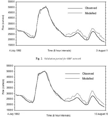
[image:5.595.58.290.90.206.2]Figures 2 and 3 present hydrographs of the RBF and MLP performance respectively. Although there appears to be little difference between the models, the statistics indicate that the RBF is generally more skilful. Close examination of these figures shows that the RBF is indeed closer to modelling the lower flows than the best MLP network. In both cases the models forecast the flood peak accurately (the respective errors in the peak flow forecasts are 1.5% and -0.6%) although both models overpredict the secondary peaks to some extent. This may occur firstly because the Table 2. Experimental results
MSRE RMSE CE AIC R-squared
(cumecs) (%)
ARMA 0.0202 4237 75.98 1674 0.91
MLP 0.0073 2068 94.24 1609 0.97
SWMLR 0.0107 2998 87.90 1607 0.97
ZOF 0.0362 6590 41.50 1759 0.49
[image:5.595.115.464.334.712.2]RBF (MQ) 0.0070 1933 94.97 1611 0.98
Fig. 2. Validation period for RBF network
Fig. 3. Validation period for MLP network
15000 20000 25000 30000 35000 40000 45000 50000 55000
Time (6 hour intervals)
Flow (cumecs)
4 July 1992 3 August 1992
Modelled Observed
Modelled Observed
4 July 1992 13 August 1992
15000 20000 25000 30000 35000 40000 45000 50000 55000
Time (6 hour intervals)
networks were trained on flood events and have had little exposure to low flow events. Secondly, the models selected for validation were based on comparisons with a flood peak in the test set (so models were chosen that predicted flood events most accurately). Thirdly, the optimisation criteria of the ANN aims to minimise the MSE. This is more sensitive to large deviations and may explain why the models have evolved to model larger flows at the expense of low flow events. An alternative would be to optimise networks with respect to, say, MSRE which would penalise models for over- or under-predicting low flow events. Further work is needed in this area.
An additional experiment was performed with the MLP to assess the effectiveness of an alternative transfer function. To this end a hyperbolic tangent function was used (this has been used in a number of previous studies; see Dawson and Wilby, 2001). However, results of this experiment provided rather disappointing results. Although the networks could be trained to model the calibration data accurately, networks utilising this transfer function were very poor at generalising and provided somewhat inaccurate forecasts when assessed with the test and validation data. In these experiments the best model that could be produced (following the same process as before) had a RMSE of 4676 cumecs for the validation data — much worse than all but the naïve ZOF model results presented in Table 2.
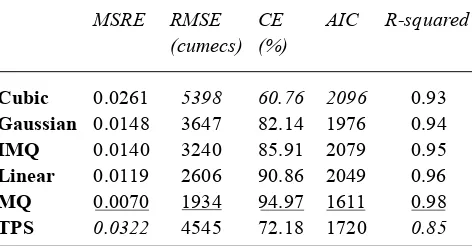
Table 3 presents the comparative performance of the RBF network using alternative transfer functions (with respect to the validation data set). The multiquadratic is the most accurate function according to all the error measures used. The results of the more ‘popular’ Gaussian function are poor by comparison and are even worse than using a simple linear function. These results emphasise the importance of using alternative transfer functions in RBF networks. Although the multiquadratic provided the most accurate model in this study, this may not be the case in all situations and all other possibilities should be explored. Further research is being
conducted by the authors into the use of alternative transfer functions and additional work is needed to explore the reasons behind their different performances.
CONFIDENCE
A criticism often levelled at neural network models is their inability to explain their reasoning and, therefore, in real time, how confident can one be in a flood forecast they have made? The authors are investigating the internal configuration of ANNs used to emulate water balance models (Abrahart et al. 2001; Wilby et al., 2002) in an attempt to explain a network’s behaviour in physical ways. An alternative technique is to provide confidence limits on the model’s behaviour calculated statistically from past performance. One possible technique is to use the standard error of the least squares regression line of observed flow on predicted flow. While this does not provide a direct measure of confidence when comparing modelled and observed data, it does provide an indirect measure that may be useful. The regression line provides a standard error measure and hence confidence intervals for the intercept and gradient of the linear regression between observed and modelled flow (Fig. 4). This can be used to investigate biases in a model’s performance. For example, in the RBF (MQ) model, the standard error of flow is 1270 cumecs. Thus, for an RBF predicted flow of 35,000 cumecs (say), one is 95% confident (1.96 standard errors about the regression line) that the actual flow that will be observed in the river in 48 hours time will be between 31,630 and 36,608 cumecs (calculating the expected flow as 34,119 cumecs from the regression line). However, for this estimate to be valid, a linear relationship must exist between the model and the observed flows and the results must be homoscedastic. While homoscedasticity can be difficult to prove, a visual inspection of these data does indicate that it is preserved in this particular case. Further work is needed to explore the validity of using this relationship in determining confidence limits.
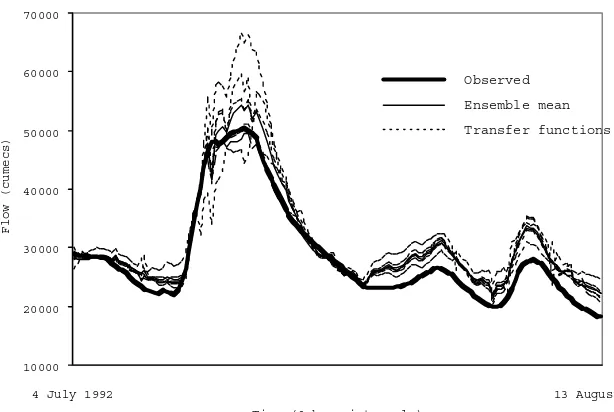
[image:6.595.46.282.611.734.2]Another way of improving confidence in a model is to combine the output from several models into a single flow estimate. This can involve coupling both conceptual and neurohydrological models. Figure 5 shows the variation in output of the RBF models with different transfer functions, along with the ensemble mean for the validation period. The figure clearly illustrates the level of uncertainty that arises from using just alternative transfer functions within the same type of neural network. This demonstrates that no single model is necessarily perfect for all conditions and shows that uncertainty surrounds any estimate. To improve estimates and confidence in predictions, it is useful, Table 3. Experimental results for different RBF transfer
functions
MSRE RMSE CE AIC R-squared
(cumecs) (%)
Cubic 0.0261 5398 60.76 2096 0.93
Gaussian 0.0148 3647 82.14 1976 0.94
IMQ 0.0140 3240 85.91 2079 0.95
Linear 0.0119 2606 90.86 2049 0.96
MQ 0.0070 1934 94.97 1611 0.98
therefore, to integrate the output from several models. This can be achieved by either selecting the output from one model, based on current conditions (for example, choose model A’s output during low flow events, and model B’s output during flood events), or integrating the predictions from the models in some way — such as averaging or weighted averaging. Various approaches have been suggested along these lines. For example, Shamseldin and O’Connor (1999) suggest using a linear transfer function model to combine model outputs; Furundzic (1998) uses a self organising map to distribute input data to alternative neural networks (each network performing ‘better’ in different conditions); and See and Abrahart (1999) propose
the use of a neural network to ‘fuse’ such outputs together. What has yet to be fully explored is the determination of confidence probabilities for combined flow forecasts. This could involve evaluating ensemble means and variance from a range of models.
[image:7.595.114.465.71.263.2]What is clear is that when predictions are made by models (be they individual or integrated models), it is important to provide some indication of the model(s)’ accuracy. By providing confidence limits on a given flow prediction, one is going some way to achieving this aim. Further work in assigning probabilities to ANN flow forecasts is currently the subject of ongoing research.
Fig. 4. Regression of observed versus modelled flow (RBF results)
Ensemble mean Observed
4 July 1992 13 August 1992
Time (6 hour intervals)
Flow (cumecs)
Transfer functions
10000 20000 30000 40000 50000 60000 70000
Fig. 5. Comparison of ensemble mean and different RBF performance
15000 20000 25000 30000 35000 40000 45000 50000 55000
Modelled Flow (cumecs)
Observed Flow (cumecs)
15000 20000 25000 30000 35000 40000 45000 50000 5500 0
0
Regression line
[image:7.595.137.444.300.506.2]Conclusions
This paper has evaluated the use of two different artificial neural network models to forecast flow in the River Yangtze, China. While the data set was somewhat limited, it was still possible to explore a number of hypotheses. Firstly, the results have shown that the popular MLP is not always the most accurate model to use and alternative network types, for example, the RBF, can prove ‘better’ in some cases. Secondly, when developing RBF networks one should not presuppose a Gaussian transfer function within the architecture. By exploring a number of alternative transfer functions the Gaussian function has been shown to under perform and, in this particular case, the multiquadratic was a significant improvement. Thirdly, the results have shown that ANNs can predict events outside their training range simply by using a limiting scaling on the data (in this case [0.1, 0.9]). Imrie et al. (2000) have explored this idea further and proposed the use of a guidance system to develop networks towards more general solutions. Finally, the importance of assigning confidence probabilities to a model’s performance has been discussed. This can be achieved in a number of ways; by evaluating a model’s past performance statistically, by exploring the internal structure of the network to provide a physical interpretation of its behaviour or by combining model outputs and computing the ensemble mean and variance of forecasts.
Acknowledgement
This work is done under a co-operation agreement between the University of Derby, UK and the Three Gorges University, China (the University of Hydraulic and Electric Engineering/Yichang was renamed as Three Gorges University in June 2000). Dawson, Wilby and Chen made a field trip to the Three Gorges area of the Yangtze River, China jointly funded by both universities. The data used in this study were provided by the Three Gorges University.
References
Abrahart, R.J., See, L. and Kneale, P.E., 1998. New tools for neurohydrologists: using network pruning and model breeding algorithms to discover optimum inputs and architectures. Proc. 3rd International Conference on Geocomputation, University of Bristol, 17-19 September.
Abrahart, R.J., Wilby, R.L. and Dawson, C.W., 2001. Inferring conceptual rainfall-runoff model processes with artificial neural networks. European Geophys.Soc. General Assembly, Nice. Bishop, C.M., 1995. Neural Networks for Pattern Recognition,
Clarendon Press, Oxford, UK.
Chinese Embassy, 1997a. Three Gorges Project in Full Swing. http://www.chinese-embassy.org.uk/Hot-Issues/Three-Gorges-Project/Press.pl-385.htm, 25 April, 2001.
Chinese Embassy, 1997b. Some facts about the Three Gorges
Project. http://www.chinese-embassy.org.uk/Hot-Issues/Three-Gorges-Project/Press.pl-gorges04.htm, 25 April, 2001. Dawson, C.W. and Wilby, R., 1998. An artificial neural network
approach to rainfall-runoff modelling. Hydrolog. Sci. J., 43, 47– 66.
Dawson, C.W. and Wilby, R.L., 2001. Hydrological modelling using artificial neural networks. Prog. Phys. Geogr., 25, 80– 108.
Dawson, C.W., Brown, M. and Wilby, R., 2000. Inductive learning approaches to rainfall-runoff modelling. Int.J. Neural Systems, 0129-0657, 10, 43–57.
Furundzic, D., 1998. Application of neural networks for time series analysis: rainfall-runoff modeling. Signal Process., 64, 383– 396.
Hall, M.J., 2001. How well does your model fit the data? J. Hydroinformatics, 3, 49–55.
Hardy, R.L., 1971. Multiquadratic equations of topography and other irregular surfaces. J. Geophys. Res., 76, 1905–1915. Haykin, S., 1999. Neural Networks A Comprehensive Foundation
(2nd edition), Prentice Hall, London.
Imrie, C.E., Durucan, S. and Korre, A., 2000. River flow prediction using artificial neural networks: generalisation beyond the calibration range. J. Hydrol., 233, 138–153.
Jayawardena, A.W. and Fernando, D.A.K., 1998. Use of radial basis function type artificial neural networks for runoff simulation. Comput. Aided Civil Infrastructure Engineering, 13, 91–99.
Jayawardena, A.W., Fernando, D.A.K. and Zhou, M.C., 1997. Comparison of multilayer perceptron and radial basis function networks as tools for flood forecasting. IAHS Publication no. 239, 173–181.
Legates, D.R. and McCabe, G.J., 1999. Evaluating the use of “goodness-of-fit” measures in hydrologic and hydroclimatic model validation. Water Resour. Res., 35, 233–241.
Maier, H.R. and Dandy, G.C., 2000. Neural networks for the prediction and forecasting of water resources variables: a review of modelling issues and applications. Environ.Modelling Software, 15, 101–123.
Mason, J.C., Tem’me, A. and Price, R.K., 1996. A neural network model of rainfall-runoff using radial basis functions. J. Hydraul. Res., 34, 537–548.
McCulloch, W.S. and Pitts, W., 1943. A logical calculus of the ideas imminent in nervous activity. Bulletin and Mathematical Biophysics, 5, 115–133.
Minns, A.W. and Hall, M.J., 1996. Artificial neural networks as rainfall-runoff models. Hydrolog. Sci. J., 41, 399–417. Nash, J.E. and Sutcliffe, J.V., 1970. River flow forecasting through
conceptual models part 1 - a discussion of principles. J. Hydrol., 10, 282–290.
Rumelhart, D.E. and McClelland, J.L. (Eds.), 1986. Parallel Distributed Processing: Explorations in the Microstructures of Cognition, Vol 1, MIT Press, Cambridge, MA.
See, L. and Abrahart, R.J., 1999. Proc. 4th Int. Conf. Geocomputation, Fredericksburg, Virginia, USA.
Shamseldin, A.Y. and O’Connor, K.M., 1999. A real-time combination method for the outputs of different rainfall-runoff models. Hydrolog. Sci. J., 44, 895–912.