Detecting dominant changes in irregularly sampled multivariate water quality data sets

https://doi.org/10.5194/hess-22-4401-2018 © Author(s) 2018. This work is distributed under the Creative Commons Attribution 4.0 License.

Detecting dominant changes in irregularly sampled multivariate

water quality data sets

Christian Lehr1,2, Ralf Dannowski1, Thomas Kalettka1, Christoph Merz1,3, Boris Schröder4,5, Jörg Steidl1, and Gunnar Lischeid1,2

1_{Leibniz Centre for Agricultural Landscape Research (ZALF), Müncheberg, Germany} 2_{University of Potsdam, Institute for Earth and Environmental Sciences, Potsdam, Germany}

3_{Institute of Geological Sciences, Workgroup Hydrogeology, Freie Universität Berlin, Berlin, Germany}

4_{Landscape Ecology and Environmental Systems Analysis, Institute of Geoecology, Technische Universität Braunschweig,}

Langer Kamp 19c, 38106 Braunschweig, Germany

5_{Berlin-Brandenburg Institute of Advanced Biodiversity Research (BBIB), Altensteinstraße 6, 14195 Berlin, Germany}

Correspondence:Christian Lehr ([email protected])

Received: 26 January 2018 – Discussion started: 16 February 2018

Revised: 29 June 2018 – Accepted: 18 July 2018 – Published: 21 August 2018

Abstract.Time series of groundwater and stream water qual-ity often exhibit substantial temporal and spatial variabil-ity, whereas typical existing monitoring data sets, e.g. from environmental agencies, are usually characterized by rel-atively low sampling frequency and irregular sampling in space and/or time. This complicates the differentiation be-tween anthropogenic influence and natural variability as well as the detection of changes in water quality which indicate changes in single drivers. We suggest the new term “domi-nant changes” for changes in multivariate water quality data which concern (1) multiple variables, (2) multiple sites and (3) long-term patterns and present an exploratory framework for the detection of such dominant changes in data sets with irregular sampling in space and time. Firstly, a non-linear dimension-reduction technique was used to summarize the dominant spatiotemporal dynamics in the multivariate wa-ter quality data set in a few components. Those were used to derive hypotheses on the dominant drivers influencing wa-ter quality. Secondly, different sampling sites were compared with respect to median component values. Thirdly, time se-ries of the components at single sites were analysed for long-term patterns. We tested the approach with a joint stream water and groundwater data set quality consisting of 1572 samples, each comprising sixteen variables, sampled with a spatially and temporally irregular sampling scheme at 29 sites in northeast Germany from 1998 to 2009. The first four components were interpreted as (1) an agriculturally induced

enhancement of the natural background level of solute con-centration, (2) a redox sequence from reducing conditions in deep groundwater to post-oxic conditions in shallow ground-water and oxic conditions in stream ground-water, (3) a mixing ra-tio of deep and shallow groundwater to the streamflow and (4) sporadic events of slurry application in the agricultural practice. Dominant changes were observed for the first two components. The changing intensity of the first component was interpreted as response to the temporal variability of the thickness of the unsaturated zone. A steady increase in the second component at most stream water sites pointed to-wards progressing depletion of the denitrification capacity of the deep aquifer.

1 Introduction

al., 2012). While the development of sensor technology, data loggers and transmission technology hopefully will help to significantly increase the number of high-frequency toring programmes in the future, most of the existing moni-toring programmes so far applied a rather low sampling fre-quency. Nonetheless, there is common agreement that for short periods with high-frequency data, longer periods of low-frequency monitoring provide invaluable context (Burt et al., 2011; Neal et al., 2012; Halliday et al., 2012; Bieroza et al., 2014). This is especially true for existing long-term records which are required as reference to distinguish be-tween natural short-term and long-term variability of the ob-served variables and the assessment of the effects of anthro-pogenic influence on water quality such as changes in land use in the catchment (Burt et al., 2008; Howden et al., 2011). The intriguing temporal and spatial variability in water quality monitoring data sets can in most cases hardly be re-lated to single causal factors. Instead, a variety of biogeo-chemical processes (e.g. Stumm and Morgan, 1996; Neal, 2004; Beudert et al., 2015), climatic (e.g. Neal, 2004) and hydrological (e.g. Molenat et al., 2008) variability and an-thropogenic influences, for example agricultural (e.g. Basu et al., 2010, 2011; Aubert et al., 2013) or forestal (e.g. Neal, 2004) land use, land use change (e.g. Scanlon et al., 2007; Raymond et al., 2008) or urbanization (e.g. Kroeze et al., 2013), interact at different scales impeding identification of clear cause–effect relationships. Usually a single solute is af-fected by numerous different drivers at different scales (see e.g. Molenat et al., 2008; Lischeid et al., 2010; Schuetz et al., 2016 for NO−₃). Inversely, a single driver usually has an impact on various solutes (Massmann et al., 2004; Lischeid and Bittersohl, 2008). This suggests that trend analyses of single variables might easily be misleading with respect to the identification of driving factors. For this purpose tech-niques which are able to account for the interaction of multi-ple drivers and observed variables are preferable.

On the other hand, despite their complexity, catchments are highly constrained systems. Usually only a few domi-nant processes determine the main dynamics of streamflow, groundwater head or water quality (Grayson and Blöschl, 2000; Sivakumar, 2004; Lischeid et al., 2016). Using joint in-formation from different solutes is an established way to de-rive hypotheses on processes or other causal factors that are dominant in the monitored data. For this purpose, dimension-reduction techniques, especially the linear principal compo-nent analysis (PCA), have been used in analyses of mul-tivariate water quality data for a long time, mostly as an exploratory tool for descriptive process identification (e.g. Usunoff and Guzmán-Guzmán, 1989; Haag and Westrich, 2002; Cloutier et al., 2008) or for determining mixing ratios (e.g. Hooper et al., 1990; Capell et al., 2011). If the anal-ysed data consist of time series of one or several variables observed at different sites, then the temporal features of the results of the dimension reduction can be analysed in a spa-tially explicit way, e.g. with respect to seasonal patterns or

long-term developments at the monitored sites (Lischeid and Bittersohl, 2008; Lischeid et al., 2010).

However, many of the methods commonly used for analysing temporal developments in monitoring data sets re-quire regularly sampled data. In practice the spatiotemporal design of sampling campaigns and monitoring networks of-ten evolves during the sampling period in an irregular way. In order to obtain a regularly sampled data set, additional in-formation with a different sampling design, e.g. from pilot studies or single sampling campaigns, might not be utilized in the analysis at all. Further irregularities in the spatiotem-poral structure of environmental monitoring data sets arise typically during the monitoring itself from a variety of rea-sons such as failure of sensors or data loggers, measurement errors, loss of samples or periods of ice or drought. Thus, in environmental monitoring practice, data sets with gaps and periods with corrupted measurements are more the rule rather than the exception (see e.g. Zhang et al., 2018, for river qual-ity data).

Lischeid et al. (2010) suggested a combination of ex-ploratory data analysis methods to detect and analyse domi-nant processes and their temporal development in multivari-ate wmultivari-ater quality data sets that is capable of dealing with irregular time series. We built on that and extended it to-wards the detection of “dominant changes” in time series of multivariate water quality data that are monitored at differ-ent sites, i.e. at differdiffer-ent parts of a catchmdiffer-ent or in differdiffer-ent catchments within a region. In analogy to the dominant pro-cess concept (Grayson and Blöschl, 2000; Sivakumar, 2004), we use the term “dominant changes” in a broad and descrip-tive sense referring to systemic changes that clearly exceed the usual range of heterogeneities in the temporal, spatial or inter-variable structure of the observed water quality data. The changes we considered as dominant were those that con-cerned (1) main components of the multivariate water qual-ity data set rather than single water qualqual-ity variables (mul-tivariate components), (2) behaviour at various sites rather than at single sites (multiple sites), and (3) long-term be-haviour rather than short-term fluctuations or single events (long-term patterns).

2 Data 2.1 Study area

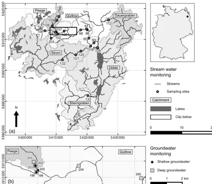
The study area is the upper part of the basin of the Ucker river located in the northeast of Germany, about 90 km north of Berlin, which drains to the Baltic Sea another 50 km fur-ther north. It is part of the Leibniz Centre for Agricultural Landscape Research (ZALF) long-term monitoring region AgroScapeLab Quillow, the LTER-D (Long Term Ecological Research Network, Germany) and the TERENO (Terrestrial Environmental Observatories, http://teodoor.icg.kfa-juelich. de, last access: 8 October 2017) Northeastern German Low-land Observatory. Water samples have been taken in the ad-jacent catchments of Dauergraben (78.9 km2), Stierngraben (104.8 km2), and Quillow (399.4 km2) with its subcatch-ments Strom (235.8 km2) and Peege (25.6 km2) (Fig. 1). At the ZALF weather station Dedelow, which is situated ap-proximately 500 m northeast of Q_97 (Fig. 1a), a mean an-nual precipitation of 550 mm and a mean anan-nual tempera-ture of 8.9◦C was observed for the hydrological years within the study period (November 1997 to October 2009). The mean annual climatic water balance for this period, calcu-lated from daily precipitation and potential evapotranspira-tion, was found to be −103 mm, exhibiting high interan-nual variability with−148 mm in the summer half year and

+45 mm in the winter half year.

The topography of the region developed basically dur-ing the Pomeranian stage and the Mecklenburgian stage of the Weichselian ice age, i.e. 15 200 to 14 100 years before present. Altitude varies from 20 m in the lowlands of the Ucker river to more than 100 m above sea level in the south-western part of the study area. During the Pleistocene, re-peated advances and recessions of the ice sheet deposited highly heterogeneous unconsolidated sediments of about 150 to 200 m thickness. The base consists of a thick Oligocene clay layer which separates the upper freshwater groundwater system from saline groundwater underneath. Based on bore-hole surveys, up to seven aquifers divided by layers of till have been identified within the unconsolidated Quaternary sediments. In some parts of the region patches of halophilous plants are found in the lowlands, indicating local upwelling of saline groundwater from the underlying Tertiary aquifer through windows of the Oligocene clay layer.

Loamy and sandy loamy soils that developed from the till substrate prevail. Most of the region is intensively used as cropland, although the fraction of arable land differs between the catchments (Table 1). Forests comprise only a minor frac-tion of the area (Table 1). Land cover did not change within the study period from 1998 to 2009. The riparian zone of the catchments is mostly used as grassland, underlain by peat and organic and sandy fluvial deposits. The hummocky landscape includes about 1300 closed drainage basins and small ponds with an area of the water surface < 1 ha (Kalettka and Rudat, 2006; Lischeid et al., 2016). Many of the larger depressions

have been connected by ditches to facilitate drainage. Partly, these ditches have later been replaced by underground pipes for land reclamation. In addition, agricultural soils are exten-sively drained by subsurface tile drainage systems. From the 13th century until the end of the 19th century, the energy of the natural water courses was also occasionally used to power mills. Today, those mills are not active any longer and have been replaced in most cases by weirs for water management or ramps. For more details on the study site, please see Merz and Steidl (2015).

2.2 Sampling and analysis

The monitoring aimed to cover the spatial and temporal vari-ability of water quality along the Quillow stream, its tribu-taries and the adjacent streams. The main focus of the moni-toring was the Quillow catchment. Here, eight sampling sites were located along the main stream and another four at each of the two tributaries Peege and Strom (Fig. 1 and Sup-plement Table S1). At the streams Dauergraben and Stiern-graben and at the Ucker river, stream water quality was mon-itored at one site respectively. Stream water sampling started in 1998 and was performed until 2009. Discharge data were only available at sites Q_93 and S_118 (Fig. 1a). Thus, we did not include it in the presented analysis. Groundwater quality was monitored in the Quillow catchment only, close to the middle reaches of the stream and close to the mouth of the Peege tributary, from 2000 to 2008 (Fig. 1b). At this site, an up to 15 m thick horizontal till layer separates a shallow and very heterogeneous unconfined aquifer from a mainly confined deep aquifer. The separating till layer crops out further downstream (Merz and Steidl, 2015). Both aquifers were monitored (Table S2). The deep aquifer is known to be confined except at well Gd_204. Groundwater level in the deep aquifer was measured daily with automatic data log-gers at wells Gd_198, Gd_201, Gd_203 and Gd_204 (Merz and Steidl, 2014a).

Groundwater quality (Merz and Steidl, 2014b) and stream water quality (Kalettka and Steidl, 2014) monitoring in the Quillow catchment covers a wide range of water quality pa-rameters. For the multivariate analysis in this study, we con-sidered from the joint groundwater and stream water quality data set only the 16 variables with less than 5 % missing val-ues, i.e. NH+₄, NO−₃, NO−₂, PO₄3−, Na+, K+, Mg2+, Ca2+, Cl−, O2, pH, water temperature, redox potential (Eh),

elec-tric conductivity (EC), SO2₄− and dissolved organic carbon (DOC) (Table S3). Each sample contained measurements of all 16 variables. Those water samples for which more than 2 of the 16 monitored variables were missing were excluded from the analysis, resulting in a set of 1572 samples. In total, 0.69 % of the values in the data set were missing. In addi-tion, we considered HCO−₃ and Fe2+concentration from the groundwater monitoring (Table S3).

0 10 20 km N

0 1 2 km

Shallow groundwater Deep groundwater Sampling sites Streams Clip below Stream water monitoring Groundwater monitoring Catchment Lakes 122 122 122 122 122 122 122 122 122122122122122122122122122122122122122122122122122122122122122122122122122122122122122122122122122122122122122122122122122122122122122122122122122122122122122122122122122122122122122122122122122122122122122122122122122

5 91 2 00 0 5 91 3 0 00

3 410 000 3 412 000 3 414 000 3416 000

Quillow Peege 5 88 0 00 0

3 400 000 3 410 000 3 420 000 3 430 000

5 89 0 00 0 5 90 0 0 00 5 91 0 00 0 5 92 0 0 00 133 133 133 133 133 133 133 133 133 133 133 133 133 133 133 133 133 133 133 133 133 133 133 133 133 133 133 133 133 133 133 133 133 133 133 133133133133133133133133133133133133133133133133133133133133133133133133133133133133133133133133133133133133133133133133133133133133133133133 Stierngraben Ucker 112 112 112 112 112 112 112 112 112 112 112 112 112 112 112 112 112 112 112 112 112 112 112 112 112 112 112112112112112112112112112112112112112112112112112112112112112112112112112112112112112112112112112112112112112112112112112112112112112112112112112112112112112112112112

Dauergraben 96 96 96 96 96 96 96 96 96 96 96 96 96 96 96 96 96 96 96 96 96 96 96 96 96 96 96 96 96 96 96 96 96 96 96 9696969696969696969696969696969696969696969696969696969696969696969696969696969696969696969696 98 98 98 98 98 98 98 98 98 98 98 98 98 98 98 98 98 98 98 98 98 98 98 98 98 98 9898989898989898989898989898989898989898989898989898989898989898989898989898989898989898989898989898989898989898 95 95 95 95 95 95 95 95 95 95 95 95 95 95 95 95 95 9595959595959595959595959595959595959595959595959595959595959595959595959595959595959595959595959595959595959595959595959595959595 ₉₃

97 100 100 100 100 100 100 100 100 100 100 100 100 100 100 100 100 100 100100100100100100100100100100100100100100100100100100100100100100100100100100100100100100100100100100100100100100100100100100100100100100100100100100100100100100100100100100100100100100100100100 102 102 102 102 102 102 102 102 102102102102102102102102102102102102102102102102102102102102102102102102102102102102102102102102102102102102102102102102102102102102102102102102102102102102102102102102102102102102102102102102102102102102102102102102102102 103 103 103 103 103 103 103 103 103 103 103 103 103 103 103 103 103 103103103103103103103103103103103103103103103103103103103103103103103103103103103103103103103103103103103103103103103103103103103103103103103103103103103103103103103103103103103103103103103103103

107 107 107 107 107 107 107 107 107 107 107 107 107 107 107 107 107 107107107107107107107107107107107107107107107107107107107107107107107107107107107107107107107107107107107107107107107107107107107107107107107107107107107107107107107107107107107107107107107107107 110 110 110 110 110 110 110 110 110 110 110 110 110 110 110 110 110 110 110 110 110 110 110 110 110 110 110110110110110110110110110110110110110110110110110110110110110110110110110110110110110110110110110110110110110110110110110110110110110110110110110110110110110110110110

104 104 104 104 104 104 104 104 104 104 104 104 104 104 104 104 104 104 104 104 104 104 104 104 104 104 104104104104104104104104104104104104104104104104104104104104104104104104104104104104104104104104104104104104104104104104104104104104104104104104104104104104104104104104 106 106 106 106 106 106 106 106 106 106 106 106 106 106 106 106 106 106 106 106 106 106 106 106 106 106 106 106 106 106 106 106 106 106 106 106 106 106 106 106 106 106 106 106 106106106106106106106106106106106106106106106106106106106106106106106106106106106106106106106106106106106106106

106 108 108 108 108 108 108 108 108 108108108108108108108108108108108108108108108108108108108108108108108108108108108108108108108108108108108108108108108108108108108108108108108108108108108108108108108108108108108108108108108108108108108108108108108108108108

109 109 109 109 109 109 109 109 109 109 109 109 109 109 109 109 109 109 109 109 109 109 109 109 109 109 109 109 109 109 109 109 109 109 109 109109109109109109109109109109109109109109109109109109109109109109109109109109109109109109109109109109109109109109109109109109109109109109109 Peege Quillow 118 118 118 118 118 118 118 118 118 118 118 118 118 118 118 118 118 118118118118118118118118118118118118118118118118118118118118118118118118118118118118118118118118118118118118118118118118118118118118118118118118118118118118118118118118118118118118118118118118118 120 120 120 120 120 120 120 120 120 120 120 120 120 120 120 120 120 120 120 120 120 120 120 120 120 120 120120120120120120120120120120120120120120120120120120120120120120120120120120120120120120120120120120120120120120120120120120120120120120120120120120120120120120120120 121 121 121 121 121 121 121 121 121 121 121 121 121 121 121 121 121 121121121121121121121121121121121121121121121121121121121121121121121121121121121121121121121121121121121121121121121121121121121121121121121121121121121121121121121121121121121121121121121121121

122 128 128 128 128 128 128 128 128 128128128128128128128128128128128128128128128128128128128128128128128128128128128128128128128128128128128128128128128128128128128128128128128128128128128128128128128128128128128128128128128128128128128128128128128128128128

Strom

(a)

(b)

Figure 1.Map of the study area. Coordinates of WGS84/UTM zone 33N are given in m.(a)Stream water monitoring sites and the location of the study area (upper Ucker river catchment) within Germany. (b)Section with the included groundwater monitoring sites. For better readability only the number of the ID of the monitoring sites is shown.

Table 1.Share of land use classes in the different catchments (percent of land cover) based on CORINE Land Cover 2000 data (DLR-DFD and UBA, 2004).

Settlements and industry Arable land Grassland Lakes Others Wetland Woodland

Dauergraben 1.7 92.1 4.1 1 0.3 – 0.8

Ucker 4.6 62.3 5.6 7.7 2.2 2.4 15.2

Stierngraben 1.4 61.2 15.8 1.2 0.9 – 19.5

Strom 2.2 54 7 6.9 1.2 – 28.7

Quillow 2.3 77 9.3 1.3 1.4 – 8.7

Peege 0 78.3 5.5 – – – 16.2

approximately monthly intervals, and groundwater samples were taken every 3 months. Median (mean) sampling inter-vals were 29 (38.7) days for stream water and 98 (125.3) days for groundwater. The one shorter sampling interval at site GdQ_198 was an exceptional sample taken during main-tenance work. In total, sampling intervals between two con-secutive samples varied between 9 and 714 days (Fig. 2).

The sites were sampled roughly similarly across seasons (Fig. 2a). The most important systematic deviations from this rule were the Peege sites and the most upstream sites of the Quillow (Figs. 2a and 1), which often fall dry in summer (Merz and Steidl, 2015).

quality data used in this article and the groundwater level data have been published under the CC-BY 4.0 license and can be found in Lehr et al. (2018) and Merz and Steidl (2014a) respectively.

3 Methods

3.1 Data preprocessing

Missing values were replaced by the median of the respec-tive variable. This concerned at most DOC (3.44 % of the values) and NO−₂ (2.54 %), whereas the percentage of miss-ing values was less than 2 % for each of the other 14 vari-ables (Table S3). Values below detection limit were replaced by 0.5 times that limit. To achieve equally weighted variables the values werez-normalized to zero mean and unit standard deviation for each variable separately.

3.2 Exploratory framework

To identify the dominant changes, we firstly used the non-linear dimension-reduction technique isometric feature map-ping (Isomap) to derive the main multivariate water quality components. To account for the interaction of groundwater and stream water, both groundwater and stream water sam-ples have been analysed together in one joint analysis. Sec-ondly, we studied differences between the sites with respect to median component values. Thirdly, we analysed the time series of the components at sites with more than 50 samples. Seasonal patterns were analysed with the Lomb–Scargle ap-proach (Lomb, 1976; Scargle, 1982„ 1989) and – if signifi-cant – were subtracted from the series prior to trend analyses. Please note that the term “seasonal” refers to the annual cy-cle throughout the articy-cle. Linear trends were estimated with the Theil–Sen estimator and tested for significance with the Mann–Kendall test. Non-linear trends were depicted with the locally weighted regression (LOESS) approach (Cleveland, 1979; Cleveland and Devlin, 1988). We then related resulting low-frequency patterns to the long-term groundwater head dynamics, likewise determined as the LOESS smooth of the de-seasonalized series. Time series analysis at different sites allowed us to check whether long-term patterns were consis-tent, pointing to more general effects in the study area.

As the methods do not require regularly sampled data in space or time, we considered every sample as additional in-formation of the spatiotemporal variability of the observed water quality in the study area rather than noise. Conse-quently, irrespective of irregularities of sampling intervals at a site or differences in sampling intervals and numbers of samples between the different sites, we included as many samples in the analysis as possible to increase the informa-tive value and support the representainforma-tiveness of the study in space and time. This might lead to a bias in the determina-tion of the components, as well as in the estimadetermina-tion of the trends of the components and their significance, if deviations

from a regular sampling scheme follow a systematic pattern. To check for that, we tested the distribution of sampling in-tervals at all sites withN >50 (Table S1) for normality with the Shapiro–Wilk test and the temporal development of the lengths of the sampling intervals for the whole observation period for monotonic trends with the Mann–Kendall test. For all tested sites a Gaussian distribution of sampling intervals as well as a monotonic trend of the length of sampling inter-vals during the observation period was rejected.

3.3 Dimension reduction

Dimension-reduction methods aim to represent a data set with a given number of dimensions (here the number of mea-sured hydrochemical variables) in a new data space with sub-stantially fewer dimensions. This is achieved by projecting the data in a new ordination system which makes a more ef-ficient use of the intrinsic structures of the data set than the original one. The axes of the new ordination system are usu-ally called components or dimensions. In the following, we will use the term “components”. For the values of a compo-nent we will use the term “scores”. The reduction of the data set’s dimensionality is achieved by considering only some of the new components for further analysis. The selection pro-cess is a trade-off between reduction of the dimensionality and minimizing the loss of potentially informative structures. Typically only the first few components are selected as they depict the main structures in the data set.

In the projection, different methods focus on different as-pects of the data. For example PCA aims at maximizing variance on the first components, classical multidimensional scaling (CMDS) at preserving the inter-point distances of the input data in the projection and self-organizing maps (SOM) at preserving the neighbourhood relations (topol-ogy) of the input data in the projection (Lee and Verleysen, 2007). In the last years, a variety of non-linear dimension-reduction methods have been developed (Van der Maaten et al., 2009). Although being sensitive to noisy data, isomet-ric feature mapping (Tenenbaum et al., 2000) was one of the best-performing approaches when applied to real-world data (Geng et al., 2005). It has been successfully applied in envi-ronmental research disciplines, e.g. biodiversity studies (Ma-hecha et al., 2007), soil sciences (Schilli et al., 2010), clima-tology (Gámez et al., 2004) and biogeochemistry (Weyer et al., 2014).

3.3.1 Principal component analysis

| | | | || | | | | | | | | | | | | | | | | | | | | | | | || | | | | | | | | | | | | | | | | | | | | | | | | | | | | | | | || | | | | || | | | | | | | | | | | | | | | | | | | | | | | | | | | | | | | | | | | | | | | | | | | | | | | || | | | | | | | | | | | | | | | | | | |

| | | || |||||| ||||| |||| ||| || | || || || | | || | | | || |||||||||| | | ||| | | || |

||| | | || ||||||| || ||||| |||||| ||| || | || || || | || | || |||| ||||||||||| | ||| | | | |||||| || |||||| ||||||||| ||| ||| ||| ||| ||| || | | | || | ||| || |||| ||||||||||| ||| ||| ||| | || ||

||| | ||||| || ||| ||||| || ||

||| || | | |||||| |||||| ||||||| ||| ||| ||| ||| |||| || || || | || |||| ||||||||||| ||| || ||| ||||| || |||||||||||| |||||| | |||||||||||| ||| ||| |||||||||||||| ||| ||||| || || || ||||| || |||| || |||| |||||||||||| ||| ||| ||| ||||| || |||||||||||| |||||| | |||||||||||||||| ||| ||||||||||||| ||| ||| ||||||||| |||||||| || |||||||||| ||||||| || | ||| |||||||||||| ||| ||| ||| ||||| || ||||||||| || |||||| | |||||||||||||||| ||| |||||||||||||| ||| ||| ||||||||| ||||||| || |||||||||| ||||||| || | ||| |||||||||||| ||| ||| ||| ||||| || |

||| ||||| || |||||||| ||| |||||| | | |||||||||||||| |||||||| ||||||||| ||| ||| ||||||||| ||||||| || |||||||||| ||||||| || | ||| |||||||||||| ||| ||| || ||||| || |||||||||||| |||||| | |||||||||||||||| ||||||||||||||||| ||| ||| ||||||||| ||||||| || |||||||||| ||||||| || | ||| |||||||||||| ||| |||

|

|||| |||||| || ||| ||||| ||| |

|| ||||| || |||||||||||| |||||| | |||||||||||||||| ||||||||| |||||| ||| ||| ||||||||| ||||||| || |||||||||| ||||||| || | ||| |||||||||||| || ||||| || |||||||||||| |||||| | |||||||||||||||| |||||||||||| |||| ||| ||| | ||||||| ||||||| || |||||||||| ||||||| || |||| |||||||||||| ||| ||| || ||||| || |||||||||||| |||||| | |||||||||||||||| |||||||| ||||||||| ||| ||||||| || |||||||||| ||||||| || | ||| |||||||||||| ||| ||| || ||||| || |||||||||||| |||||| | |||||||||||||||| |||||||| ||||||||| ||| ||| ||||||||| ||||||| || |||||||||| ||||||| || | ||| |||||||||||| ||| |||

1998 2000 2002 2004 2006 2008

| | | | || | | | | | | | | | | | | | | | | | | | | | | | || | | | | | | | | | | | | | | | | | | | | | | | | | | | | | | | || | | | | || | | | | | | | | | | | | | | | | | | | | | | | | | | | | | | | | | | | | | | | | | | | | | | | || | | | | | | | | | | | | | | | | | | |

| | | || |||||| ||||| |||| ||| || | || || || | | || | | | || |||||||||| | | ||| | | || |

||| | | || ||||||| || ||||| |||||| ||| || | || || || | || | || |||| ||||||||||| | ||| | | | |||||| || |||||| ||||||||| ||| ||| ||| ||| ||| || | | | || | ||| || |||| ||||||||||| ||| ||| ||| | || ||

||| | ||||| || ||| ||||| || ||

||| || | | |||||| |||||| ||||||| ||| ||| ||| ||| |||| || || || | || |||| ||||||||||| ||| || ||| ||||| || |||||||||||| |||||| | |||||||||||| ||| ||| |||||||||||||| ||| ||||| || || || ||||| || |||| || |||| |||||||||||| ||| ||| ||| ||||| || |||||||||||| |||||| | |||||||||||||||| ||| ||||||||||||| ||| ||| ||||||||| |||||||| || |||||||||| ||||||| || | ||| |||||||||||| ||| ||| ||| ||||| || ||||||||| || |||||| | |||||||||||||||| ||| |||||||||||||| ||| ||| ||||||||| ||||||| || |||||||||| ||||||| || | ||| |||||||||||| ||| ||| ||| ||||| || |

||| ||||| || |||||||| ||| |||||| | | |||||||||||||| |||||||| ||||||||| ||| ||| ||||||||| ||||||| || |||||||||| ||||||| || | ||| |||||||||||| ||| ||| || ||||| || |||||||||||| |||||| | |||||||||||||||| ||||||||||||||||| ||| ||| ||||||||| ||||||| || |||||||||| ||||||| || | ||| |||||||||||| ||| |||

|

|||| |||||| || ||| ||||| ||| |

|| ||||| || |||||||||||| |||||| | |||||||||||||||| ||||||||| |||||| ||| ||| ||||||||| ||||||| || |||||||||| ||||||| || | ||| |||||||||||| || ||||| || |||||||||||| |||||| | |||||||||||||||| |||||||||||| |||| ||| ||| | ||||||| ||||||| || |||||||||| ||||||| || |||| |||||||||||| ||| ||| || ||||| || |||||||||||| |||||| | |||||||||||||||| |||||||| ||||||||| ||| ||||||| || |||||||||| ||||||| || | ||| |||||||||||| ||| ||| || ||||| || |||||||||||| |||||| | |||||||||||||||| |||||||| ||||||||| ||| ||| ||||||||| ||||||| || |||||||||| ||||||| || | ||| |||||||||||| ||| |||

Sampling date

GdP_203 (25) GdP_201 (25) GsP_202 (11) GdQ_198 (28) GsQ_199 (18) GsP_200 (6) GdQ_204 (25)

GdQ_205 (2) P_110 (51)

P_109 (8) P_108 (61) P_107 (78) Q_103 (8) Q_102 (11) Q_106 (12) Q_104 (71) Q_100 (110) Q_98 (127) Q_97 (126) Q_96 (11) Q_95 (125) Q_93 (126) S_122 (1) S_121 (23)

S_120 (1) S_118 (118) St_133 (124) U_128 (114) D_112 (126)

● ●

● ●

● ●

● ●

●

● ● ● ●●● ● ●

● ●

●● ● ● ●●

●● ●●●●● ● ● ●

●●● ●●●●●●

●● ● ●●●●●●

●● ● ●●●●●●●

●● ● ●●●●●

●

● ●

●● ● ●●●● ●

●● ● ●●●●●●●

●● ● ●●●●

●● ● ●●●●●

0 50 100 150

Days between subsequent sampling dates (b)

(a)

Figure 2. (a)Sampling dates at the sites for the whole monitoring period.(b)Box plots of the variability of sampling intervals during the monitoring period. For better readability, the maximum of thexaxis is limited to 180 days. The median (red) and mean (blue) of sampling intervals are shown separately for the groundwater and stream water sites. Grey vertical lines mark the 1-day, 1-week and 1-month interval. (a, b)The dashed horizontal line separates groundwater sites (bottom) from stream water sites (top). Labels: P, Peege; Q, Quillow; S, Strom; St, Stierngraben; U, Ucker; D, Dauergraben; Gs, shallow groundwater; Gd, deep groundwater. The number of samples at each site is given in brackets. Names of the sites with more than 50 samples are printed bold.

to successively maximize the variance of the data set on the new calculated components. The scores of the com-ponents are calculated as weighted linear combinations of the original variables. The weights (loadings) of the linear combination define the axes of the data space in which the data are projected. The loadings are the eigenvectors de-rived from an eigenvalue decomposition of the covariance matrix of the analysed variables. If the analysed variables arez-normalized, as was done here, their covariance matrix is equivalent to the (Pearson) correlation matrix. The com-ponents are ordered with decreasing size of their eigenval-ues. The share of variance that is assigned to a component is proportional to the size of its eigenvalue in relation to the sum of all eigenvalues. Thus, the ratio of total variance that is captured by the considered components gives a measure of performance of the PCA. PCA was performed in R (R Core Team, 2017) with the function “princomp” of the de-fault package “stats”.

3.3.2 Isometric feature mapping

Isometric feature mapping (Isomap) is a non-linear extension of CMDS. It aims to approximate the global non-linearity in

a data set by local linear fittings (Geng et al., 2005). This is done by mapping approximated geodesic inter-point dis-tances to an Euclidean distance matrix via a neighbourhood graphG(Tenenbaum et al., 2000). The geodesic distance be-tween two points is the distance along the surface of a (non-linear) manifold, in contrast to the straight-line Euclidean distance (Geng et al., 2005). The neighbourhood graph G

consists of segments that connect every data point to its k

the neighbourhood graph G is embedded in the Euclidean space.

In contrast to PCA, assessing performance based on the eigenvalues of the components is not applicable for Isomap. Performance of the dimension reduction of the Isomap ap-proach was assessed and compared to performance of the PCA by the squared Pearson correlation coefficient (R2) of the inter-point distances in the high-dimensional data space and in the low-dimensional projection spanned by selected components (Lischeid and Bittersohl, 2008; Lischeid et al., 2010). A perfect fit would yield a value of 1 and a value of 0 reflects no correlation between the distance matrices of the original data and of the projection. Please note that with this measure the contribution of single components to the over-all performance does not necessarily decrease monotonicover-ally with increasing order of the components, as it is the case for the eigenvalue-based performance measure of PCA. For the local assessment of the representation of inter-point distances at the individual sites, only the data points from the respec-tive sites were used. Because the selection of data points at a site is only a subset of the global data set for which the di-mension reduction was performed, the performances regard-ing the representation of inter-point distances differ between the individual sites as well as compared to the overall perfor-mance for the global data set. At some sites it can even hap-pen that adding more components does not improve the rep-resentation of inter-point distances in the low-dimensional projection for every component. Isomap and the determina-tion of the distance matrices were performed with the R pack-age “vegan” (Oksanen et al., 2017).

3.3.3 Interpretation of components

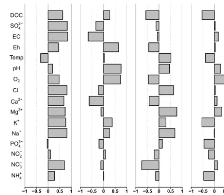
The analysis focused on those components that explained a major fraction of the total inter-point distances. The consid-ered components were regarded to reflect dominant drivers influencing water quality. Here, the term “driver” was used for biogeochemical and hydrological processes as well as for anthropogenic influences affecting water quality. Corre-spondingly we formulated a hypothesis for each considered component. The interpretation of the components is based on analysing (i) the correlations between measured variables and component scores as well as (ii) spatial and temporal patterns of the scores.

Correlation between scores of a selected component cpx

and values of single variables might be blurred due to the effects of other components on the same variable. We ex-cluded those effects by analysing the relationships between scores of the selected component cpxand the residuals of the

multiple linear regression (mlr) of the single variable vi at

hand and the remaining other considered components CP\x

(residuals):

cor(cp_x,residualsmlr(vi,CP\x)

), (1)

where CP\xis the set of m considered components, without the selected component cpx; andβ0andβj are the intercept

and coefficients of the regression

mlr(vi,CP\x)=β0+6j∈{CP\x}βjcpj+residuals. (2)

To assess the relationships between components and residu-als we used bivariate scatterplots. To summarize the relation-ships between components and residuals we used the Spear-man rank correlation, which enables us to consider non-linear relationships as well, as long as they are monotonic. In addition, it is less sensitive to extreme values than the Pear-son correlation.

3.4 Time series analysis

At sites with more than 50 samples, time series of compo-nent scores were analysed for seasonal patterns, linear trends and non-linear trends. The sites were compared with respect to the identified long-term patterns to detect general patterns in the study area. The significance level for trend and fre-quencies in this study was set top≤0.05. At each site, the fractions of variance of a time series that were assigned to its seasonal pattern, linear trend or non-linear trend were deter-mined as theR2of the respective pattern with the component series. In the case of significant seasonal patterns, the estima-tions of the trends were based on the de-seasonalized series. Accordingly, the fractions of variance assigned to the trends were determined as theR2of the trend pattern with the de-seasonalized series. The decomposition of the time series in a seasonal component and a non-linear trend derived with LOESS was inspired by the seasonal-trend decomposition procedure based on LOESS (STL) of Cleveland et al. (1990). 3.4.1 Lomb–Scargle method

Standard Fourier analysis requires an equidistant time se-ries, which was not given in our study. Therefore, the esti-mation of seasonal patterns in the time series was done with the Lomb–Scargle method, which is an extension of Fourier analysis to the unevenly spaced case genuinely invented in astrophysics (Lomb, 1976; Scargle, 1982). The application of the Lomb–Scargle method in this study follows to a large ex-tent the workflow suggested by Glynn et al. (2006) as well as Hocke and Kämpfer (2009). Details are given in Appendix A. The implementation used in this paper can be accessed as an R script at https://doi.org/10.4228/ZALF.2017.340 (Lehr et al., 2018).

not necessarily linear. Being based on rank correlation, data do not have to obey any specific distribution. Please note that we did not account for the effect of overestimation of the sig-nificance of trends with the Mann–Kendall test due to short-term autocorrelation (Yue et al., 2002). That would have re-quired an assessment of the lag-1 autocorrelation which was hampered by the irregular sampling. Neither did we con-sider long-term memory and its effects on the statistical sig-nificance of the trends (Cohn and Lins, 2005; Zhang et al., 2018). Consequently, we did not consider the possible ef-fects of the irregular sampling on the long-term memory (fractal scaling) of the water quality series either (Zhang et al., 2018). Due to the limited number of samples per year and non-equidistant sampling, the seasonal Mann–Kendall test was not applicable (Fig. 2). Instead, significant seasonal patterns according to the Lomb–Scargle approach were sub-tracted prior to trend analysis. The Mann–Kendall test was performed with the R package “Kendall” (McLeod, 2011).

3.4.3 Locally weighted regression (LOESS)

We assessed non-linear trends and low-frequency patterns with locally weighted regression (LOESS; Cleveland, 1979; Cleveland and Devlin, 1988), where the smoothing is done by local fitting of a second-order polynomial to each point

x in the data set using weighted least squares. The weights for each value to be fitted are scaled to the range from 0 to 1 by the distance d(x) between x and its qth closest point. The ratio of q to the number n of all data points, i.e. the span of the local regression smoother, defines the degree of smoothing. We used the default smoothing span, which is a proportion of q/n=0.75 ofx’s nearest neigh-bours. Data points further away than the qth data point do not contribute to the regression. Within the range of the span, the weights wi of the neighbouring points xi in the

least squares fit decrease with increasing distance of xi to

x symmetrically aroundx according to the tricubic weight-ing function wi(x)=(1−[|xi−x|) /d (x)]3)3. Again,

sig-nificant seasonal patterns according to the Lomb–Scargle ap-proach were subtracted prior to trend analysis. For details about choosing different LOESS parametrizations, please see Cleveland (1979) as well as Cleveland and Devlin (1988). Local extrema of the LOESS smooth were identified with the R package “EMD” (Kim and Oh, 2009, 2014.).

4 Results

4.1 Multivariate components

We achieved the best performance of the Isomap dimension reduction withk=1300 (Table 2). In the following, results are presented for the first four Isomap components represent-ing 88 % of the inter-point distances of the total data set. For single sites (with more than 15 samples), between 29 % and

−1 −0.5 0 0.5 1 Comp 1 NH4

+

NO3 −

NO2 −

PO4 3−

Na+

K+

Mg2+

Ca2+

Cl−

O2

pH Temp

Eh EC SO4 2−

DOC

−1 −0.5 0 0.5 1 Comp 2

−1 −0.5 0 0.5 1 Comp 3

−1 −0.5 0 0.5 1 Comp 4

Figure 3.Spearman rank correlation of a component and the resid-uals of the multiple linear regression of the measured variable and the remaining three other components.

97 % of the respective inter-point distances were represented (Table S4).

The first component depicted 42 % of the inter-point dis-tances of the total data set. Plotting residuals of the variables versus the first component showed strong positive correla-tions for NO−₃, Na+, K+, Mg2+, Ca2+, Cl−, EC, SO2₄−, DOC and slightly weaker, but still positive, correlations for O2and

Eh. Temperature was the only variable correlating negatively with the first component (Fig. 3). Visualization of the compo-nent scores versus residuals of solute concentration revealed predominantly linear relationships (Fig. S1 in the Supple-ment).

The second component reflected 18 % of the inter-point distances in the data. It exhibited clear positive correlation with O2 concentration, pH and Eh, and weaker correlation

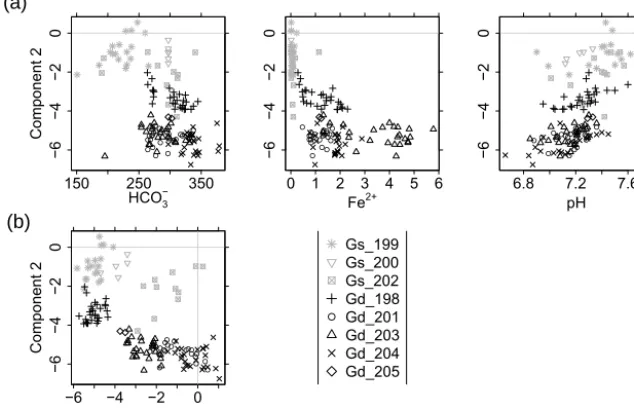
with Na+, K+ and DOC. It was inversely correlated with Ca2+, EC and SO2₄− (Figs. 3 and S2). In the groundwa-ter samples, HCO−₃ and Fe2+ had been determined as well. Both solutes were negatively correlated with this component (Fig. 4a). NO−₃ concentration in the deep groundwater sam-ples was very low (with 27 % of the samsam-ples below detection limit) and did not show any clear correlation with the second component. Low component scores in the groundwater came along with high Ca2+and HCO−₃ concentration.

The relationship of scores of component one and two in the groundwater is shown in Fig. 4b. Except for the two shal-low wells close to the Peege stream (Gs_200, Gs_202; see Fig. 1b), scores of the first and second component are nega-tively related (Fig. 4b).

150 250 350

−6

−4

−2

0

HCO₃−

Component 2

● ● ●

● ● ● ● ● ● ● ● ●

● ● ●●

● ●

● ●●

● ● ● ●

0 1 2 3 4 5 6

−6

−4

−2

0

Fe2+

● ● ●

● ● ●● ●●●●● ● ● ● ●

●● ●

● ● ● ● ● ●

6.8 7.2 7.6

−6

−4

−2

0

pH

● ●●

● ● ●●●●

● ● ●● ●

● ●

● ● ●

● ●

● ●● ●

−6 −4 −2 0

−6

−4

−2

0

Component 1

Component 2

● ● ●

● ● ●●●● ● ● ●

●● ●●

● ●

● ● ● ● ● ● ●

●

Gs_199 Gs_200 Gs_202 Gd_198 Gd_201 Gd_203 Gd_204 Gd_205 (a)

(b)

Figure 4. (a)Selection of variables versus scores of component 2 for the groundwater samples. Concentration in mg L−1.(b)Scores of component 1 versus component 2 at the groundwater sites.

correlations were found for NO−₃, Ca2+, O2, Eh and DOC

(Figs. 3 and S3).

Another 22 % of the inter-point distances in the data were assigned to the fourth component. Residuals of the compo-nent scores showed negative correlation for NH+₄, PO3₄−, K+, temperature, and DOC and positive correlation for O2 (Figs. 3 and S4). The range of component values was

spanned mainly by single large values of NH+₄, PO3₄− and K+that cannot be explained with the preceding three compo-nents (Fig. S4). This highlights the importance of particular events for the fourth component.

4.2 Multiple sites

Median values of scores of the first component clearly dif-fered between streams (Fig. 5a). At the Strom sites, the me-dian score values were considerably lower than those from the other stream water sampling sites. The median values of scores of the sites at the Quillow and Stierngraben showed intermediate values followed by the Ucker site, the Peege sites and finally the Dauergraben with the highest median score value. Groundwater samples in general exhibited con-sistently low scores for the first component, but without clear differences between deep and shallow groundwater samples. Mixing of water from different streams was visible at site Q_93 downstream of the confluence of the Quillow (Q_95) and of the Strom stream (S_118), as well as at site Q_100 downstream of the confluence of Q_104, Q_102 and P_107 (Figs. 1 and 5a).

Stream water samples exhibited the highest scores of the second component, whereas low scores were limited to deep groundwater samples, and shallow groundwater

sam-ples were in an intermediate position (Fig. 5b). Median val-ues of the stream water sites were approximately on the same level except for the sites Q_103, Q_106 and U_128, which exhibited noticeably higher median values than the other stream water sites, and the two Peege sites P_109 and P_108, which exhibited median values on the same level as the shal-low groundwater sites Gs_199 and G_200. The scores in the deep groundwater clearly showed the largest absolute values, indicating the significance of deep groundwater for this com-ponent (Fig. 5b).

Scores of the third component in the deep groundwater were consistently higher than in shallow groundwater, while the stream water samples covered the whole range of val-ues (Fig. 5c). The lowest scores of the third component were found at the Peege sites and in the shallow groundwater, and the highest scores were found at Ucker, Dauergraben and the deep groundwater. At the Quillow stream, scores tended to increase from the spring to the outlet. The effect of mixing of tributaries with different water qualities was visible along the course of the Peege and Quillow streams downstream of the respective confluences at the sites P_108, Q_95 and Q_93 (Figs. 1 and 5c).

The range of values of the fourth component was strongly biased towards negative values, caused by single events at some sites which exhibited very low values (Fig. 5d).

4.3 Long-term patterns

pat-Table 2.CumulatedR2of the reproduction of the inter-point distances of the data in the projection by the first ten components of the best Isomap run and linear PCA.

Component 1 2 3 4 5 6 7 8 9 10

Isomap 0.42 0.6 0.66 0.88 0.94 0.96 0.97 0.98 0.98 0.99

PCA 0.39 0.57 0.65 0.88 0.94 0.95 0.97 0.98 0.99 0.99

● ● ● ● ● ● ● ● ● ● ● ● ● ● ● ● ● ● ● ● ● ● ● ● ● ●●● ● ● ● −5 0 5 10 Component 1

Groundwater Stream water

(a) ● ● ● ● ● ● ● ● ● ● ● ● ● ● ● ● ● ● ● ● ● ● ● ● ● ● ● ● ● ● ● ● ● ● ● ● ● ● ● ● ● ● ● ● ● ● ● ● ● ● −4 0 4 Component 2 (b) ● ● ● ● ● ● ● ● ● ● ● ● ● ● ● ● ● ● ● ● ● ● ● −4 0 4 Component 3 (c) ● ● ● ● ● ● ● ● ● ● ● ● ● ● ● ● ● ● ● ● ● ● ● ● ● ● ● ● ●●● ● ● ● ● ● ● ● ● ● ● ● ● ● ● ● ● ● ● ● ● ● ● ● ● ● ● ● ● −20 −10 0

Gd_203 Gd_201 Gs_202 Gd_198 Gs_199 Gs_200 Gd_204 Gd_205 P_110 P_109 P_108 P_107 Q_103 Q_102 Q_106 Q_104 Q_100 Q_98 Q_97 Q_96 Q_95 Q_93 S_122 S_121 S_120 S_118 St_133 U_128 D_112

Component 4

~ ~ x ~ ~ ~ ~ ~ x x

(d)

Figure 5.Box plots of scores of component 1 to 4 at different sites. Sites withN <13 are marked with “∼”, those withN <3 with “X”. Labels: P, Peege; Q, Quillow; S, Strom; St, Stierngraben; U, Ucker; D, Dauergraben; Gs, shallow groundwater; Gd, deep groundwater.

terns had a period length in the range between 350 and 380 days. For de-seasonalization these seasonal patterns were subtracted from the time series prior to analysis for linear and non-linear trends.

Most of the time series of the scores of the first compo-nent exhibited clear seasonal patterns with maximum scores during the winter season (Figs. 6 and 7). Between 30 % and 67 % of the variance was assigned to the seasonal pattern. At all sites we found significant negative monotonic trends (Fig. 6). The strongest decline was found at site D_112 and the weakest trend at site Q_97 (not shown). The linear trend comprised between 9 % and 48 % of the variance of the de-seasonalized time series (Fig. 6). In contrast, the LOESS smooth depicted 14 % to 57 % of the variance (Fig. 6). It showed a decrease until December 2004 approximately and an increase thereafter (Fig. 8). The de-seasonalized time

se-ries of groundwater heads showed a similar behaviour, with the minimum water level in June 2006 (Fig. 8). Timing of the minimum values of the scores of the first component varied between sites, spanning a range from 17 February 2004 to 17 March 2009 (Fig. 8). As an example, Fig. 7 gives the time se-ries of scores of the first component at site Q_93, the seasonal pattern extracted from the series and the de-seasonalized time series with the non-linear trend estimated with the LOESS smoother.

Unlike for the first component, only 5 of the 13 consid-ered time series of the second component exhibited a clear significant seasonal pattern, accounting for 17 % to 48 % of the variance (Fig. 6). The maxima of the seasonal patterns of the sites at Quillow and Ucker were in spring and at Stiern-graben and DauerStiern-graben in summer. In contrast, significant monotonic trends were found at most of the stream water sampling sites. All significant trends of the second compo-nent were positive. The linear trend comprised between 5 % and 16 % of the variance of the time series, while the LOESS smooth comprised between 4 % and 25 %.

Values of the third component showed a clear seasonal pattern with maxima in summer (Fig. 6). Between 30 % and 60 % of the variance was assigned to the seasonal signal. The only exception was site D_112 were the seasonal pattern was distorted by strong maxima in the winters of 2003, 2004 and 2007. Only at four sites were significant linear trends found. All of them were negative, comprising between 6 % and 13 % of the variance. The LOESS smooth depicted between 0 % and 21 % of the variance.

For the fourth component, significant seasonal patterns with maxima in summer were observed at 7 of the 13 anal-ysed series, comprising between 17 % and 61 % of the vari-ance (Fig. 6). Five sites showed a significant monotonic trend, comprising between 5 % and 10 % of the variance. A negative trend was observed at site St_133 only. Four sites showed a positive trend. The LOESS smooth depicted be-tween 1 % and 16 % of the variance.

5 Discussion

5.1 Multivariate components

0 0.5 1 Comp 1 − − − − − − − − − − − − − P_110 (51) P_108 (61) P_107 (78) Q_104 (71) Q_100 (110) Q_98 (127) Q_97 (126) Q_95 (125) Q_93 (126) S_118 (118) St_133 (124) U_128 (114) D_112 (126)

0 0.5 1 Comp 2 + + + + + + + + + +

0 0.5 1 Comp 3

− − − −

0 0.5 1 Comp 4 + + − + + Seasonal pattern Theil−Sen estimator LOESS smooth

Figure 6.Fraction of variance of the time series of the Isomap com-ponent scores of sites withN >50 assigned to the seasonal pattern (dark grey) and the trend estimated by the linear Theil–Sen estima-tor (mid-grey) as well as the non-linear LOESS smooth (light grey). Fraction of variance is derived as theR2 of the scores of the re-spective component with the seasonal pattern or the estimated trend. Only significant seasonal patterns and linear trends are shown. The sign of the linear Theil–Sen estimator is given in the respective line. The number of samples at each site is given in brackets.

set. As there were only minor differences, we will present in the following the results of Isomap only.

For PCA and Isomap, the first component represents by definition the correlation structure that predominantly can be extracted from the set of variables as a whole. If all the load-ings of the first component of a PCA have the same sign, it is a weighted average of all the analysed variables (Jolliffe, 2002; Jolliffe and Cadima, 2016). The stronger the analysed variables are linearly correlated, the more the first compo-nent approximates the arithmetic mean of all variables (for examples with hydrometric data see Lischeid, et al., 2010; Lehr et al., 2015). Furthermore, the first component serves as reference for all the subsequent components.

In this study each sample of the multivariate water quality data set is uniquely defined by a sampling site and a sampling date. Thus, the first component depicted (a) for each sam-pling site the pattern that was most prominent in the time se-ries of the variables correlating with the first component and (b) between the sampling sites the difference in concentration level of those variables. High values of the first component indicate synchronous appearance of relatively high Eh and EC together with relatively high concentration of NO−₃, Cl−,

−3 −2 −1 0 1 2 Comp 1 ● ● ● ● ● ● ● ● ● ● ● ● ● ● ● ●● ● ● ● ● ● ● ● ● ● ● ● ● ●● ● ● ● ● ● ● ● ●● ● ● ● ● ● ●● ● ● ● ● ● ● ● ● ● ● ● ● ● ● ●●● ● ●● ● ● ● ● ●● ● ● ● ● ● ● ● ● ● ● ● ● ● ● ● ● ● ● ●● ● ● ● ●● ● ● ● ● ● ● ● ● ● ● ● ●● ● ● ● ● ● ● ● ● ● ● ● ● ● ● ● Period [days]: 368

● ● ● ● ● ●● ● ● ● ● ● ●● ● ●●● ● ● ● ● ● ●● ●● ●●● ● ● ● ● ● ●● ● ●● ●●● ● ● ●● ● ● ●● ● ● ● ● ● ● ● ● ● ●● ●● ● ● ● ● ● ●● ● ● ● ● ● ● ● ● ● ● ● ●● ● ● ●● ●●● ●● ● ●●● ● ● ●● ● ● ● ● ● ● ● ● ● ● ● ● ●● ● ● ● ● ●●● ● ● ● ●

1998 2000 2002 2004 2006 2008

−3 −2 −1 0 1 D e-s ea so na liz ed c om p 1 LOESS ● ● ● ● ● ●● ● ● ● ● ● ●● ● ●●● ● ● ● ● ● ●● ●● ●●● ● ● ● ● ● ●● ● ●● ●●● ● ● ●● ● ● ●● ● ● ● ● ● ● ● ● ● ●● ●● ● ● ● ● ● ●● ● ● ● ● ● ● ● ● ● ● ● ●● ● ● ●● ●●● ●● ● ●●● ● ● ●● ● ● ● ● ● ● ● ● ● ● ● ● ●● ● ● ● ● ●●● ● ● ● ● (a) (b)

Figure 7. (a)Time series of scores of the first component at site Q_93 (N=126) in black and the seasonal pattern estimated with Lomb–Scargle in grey.(b)The de-seasonalized series in black and the non-linear trend estimated with LOESS in grey.

−2 0 2 4 6 Component 1 64 66 68 70

2000 2002 2004 2006 2008

Groundw

ater le

vel in m a.s

.l. ● Gd_198 ● Gd_201 ● Gd_203 ● Gd_204 ● ●● ●●●●●● ●●●●● ●●●● ●●●●● ●●● ●● ●● ● ● ●● ● ● ● ●● ●●●●●●●●●● ● ● ●●●● ● ●● ●●●●●●● ●● ●●●●● ●●●●● ● ●●● ●● ● ●● ●● ●● ● ●● ● ●● ●●●● ●●●●●●●● ●●● ● ●●● ● ● ●●●●●●● ●●●● ●●●● ●●●● ●●●●● ●●● ●●●●●● ●●● ●●● ●● ●● ● ●● ●●●● ● ● ●●●●●●●●●● ●●●●● ●●● ●●● ●●● ●● ●● ●●●●●● ●●●●●● ●●●●●●● ●●● ●●● ●●● ●●● ●●●● ●● ●● ●● ● ●● ●●●● ●●●●●●●●●●● ●●●●● ●●●●●●●●●● ●● ●●●●●●●●●●_{●●●●●●} ● ●●●●●●●●●●●● ●●● ●●●_{●●●●●●●●●●●●●● ●●●} ●●●●● ●● ●● ●● ●●●●● ●● ●●●●●● ●●●● ●●● ●●●●●●●●● ●●●●●● ●●● ●●●●● ●● ●●●●●● ●●●●●● ●●●●●● ● ●● ●●●●●●_●●●● ●●●_{● ●●●} ●●●●_{●●●●●} ●●●● ●●● ●●● ●●●●●●●●● ●●●●●●●●●● ●●●●●●● ●●● ●●●●●●● ●● ●●●● ●●●●●●● ●●●●● ●●● ●●● ●●● ●●●●● ●●●●●●●●●●●_{●● ●●●●} ●● ● ●●●●●●●●●●●●●●●●_{●●● ●●} ●●●●_{●●●●●} ●●● ●●● ●●● ●_{●●●●●●●● ●●●●●●● ●● ●●●●●}●●●●●●●●●●●● ●● ●●●● ●●●● ●●●●●●●●●●●●●● ●●●●●●●● ●● ●●●●●●● ●●●● ●●●●●● ● ● ●●●_●●●● ●●●_{●●●●●●●●} ●●●●●●●● ●●●●●●●● ●● ● ●●● ●●●●●● ●●●●●●● ●●●●●●●●●●●●●●●●● ●● ●●●●●●●●●●●●●● ●●●●●●● ●●● ●●●● ●●●●● ●●●●● ●●●●●●● ●● ●●●● ● ●● ●●●●●●●●●●_●●●● ●●●●●●●●_{●●●●●} ●●●● ●●● ●●● ●●●●●●●●● ●●●●●●● ●● ●●●●●●●●●●●●●● ●●●●●●●●● ●●●●●●● ●●●●● ●●● ●●● ●● ●●●●● ●●●●●●●●●●●●●● ●●●●●● ● ●●●●●●●●● ●●●●●●● ●●●●●●●●●_{●●●●●● ●●} ● ●●● ●●●●●●●●● ●●●●●●● ●● ●●●●●●●●●● ●●●●●●● ●● ●●●● ●●●●●●●●●●●● ●●●●●● ● ●● ●●●● ●●●●● ●●● ●●●●●●●●●●● ●●●●● ●●●●●●● ●●●●●●_{●●●●●} ● ●●●●●●● ●● ● ● ●●●●●●●●●●●●●● ●● ●●●●●●●●●● ●●●●●●● ●● ●●●_{● ●●●●●●●●●●●● ●●● ●●●} ●●●● ●●● ●● ●●●●●● ●●●● ●●●●●● ●● ● ●●● ●●●●●● ●●●●●●● ●●● ●●●●●●●●_●●●● ●● ●●● ●●●●●●● ●●●●●●●●●●●● ●●●●●●● ●● ●●●● ●●●●●●●●●●●● ●●● ●●● ●● ●● ● ●● ●● ●● ●●●●●●●●●●●●●● ●● ●●●● ●● ●●●●●●●●●● ● ●●● ●●●●●● ●●●●●●●●●●● ●●● ●●● ●●●●●● ●●●●●●●●●●● ●●●●●●●● ●●●● ●●●●●●●●● ●●●●●●●●● ●●●●●●●●● ● P_110 ● P_108 ● P_107 ● Q_104 ● Q_100 ●

Q_98●Q_97

● Q_95 ● Q_93 ● S_118 ● St_133 ● U_128 ● D_112

Figure 8.Left y axis: LOESS smooth of time series of the first component at sites withN >50 in grey. If a significant seasonal pattern was present, this was removed before smoothing. Righty

SO2₄−, Na+, K+, Mg2+, Ca2+, DOC and O2 accompanied

with relatively low temperature (Fig. 3).

The whole study region is characterized by relatively in-tense agriculture (Table 1). Thus, in addition to the natural background, we assume a general effect of the agricultural practice on the solute concentration level and the dynamics of the water quality series in the area. Enhanced concentra-tion of NO−₃, Cl−, SO2₄− and Ca2+ is typical for ground-water and stream ground-water in regions with intense agriculture compared to forested areas (Broers and van der Grift, 2004; Fitzpatrick et al., 2007; Lischeid and Kalettka, 2012). Nitro-gen and potassium are the main ingredients of mineral fer-tilizers. Cl− and SO2₄− are the dominating anions in potas-sium fertilizers. SO2₄− is a major ingredient of phosphorus fertilizers and in some nitrogen fertilizers. Calcite is present in some nitrogen fertilizers or is applied separately via lim-ing. DOC might be leached from slurry application or via tile drains after mechanical destruction of topsoil aggregates during tillage (Graeber et al., 2012). In addition, cations from the soil matrix might be leached by an enhanced anion con-centration (mainly NO−₃) (Jessen et al., 2017). Overall the application of fertilizers and other agricultural practices like tillage tend to enhance the solute concentration of seepage water (Pierson-Wickmann et al., 2009). Thus, we interpreted the first component as the enhancement of the natural back-ground level of solute concentration due to agricultural prac-tices.

Compared to the first component, the relationships of the second component with Eh, pH and O2 concentration were

more clearly expressed (Figs. 3 and S2). The range of the scores of the second component was spanned by the lowest values in the deep groundwater and the highest values in the stream water (Fig. 5b), whereas shallow groundwater exhib-ited intermediate scores. This sequence corresponds to redox conditions expected in those water categories. Thus, we in-terpreted the second component as a redox-controlled com-ponent covering a sequence from reducing conditions in deep groundwater to post-oxic conditions in shallow groundwater and oxic conditions in stream water. O2and NO−₃

concentra-tion in deep groundwater samples usually was below the de-tection limit, which is a common feature in this region (Merz et al., 2009). NO−₃ in seepage and groundwater can be deni-trified by microorganisms which use the oxidation of sulfides to sulfate as electron donor for denitrification (Massmann et al., 2003; Jørgensen et al., 2009). We ascribed the high SO2₄− and Fe2+ concentration to the oxidation of pyrite (Figs. 4a and S2). Pyrite and other sulfides are abundant in the Pleis-tocenic sediments of northern Germany (e.g. Weymann et al., 2010). Consequently, the pH decreases, calcite gets dissolved and the HCO−₃ concentration increases. Part of the released Ca2+replaces Na+and K+being sorbed to clay minerals.

We interpreted the clear separation in the third compo-nent between relatively low scores for the shallow aquifer and relatively high scores for the deep aquifer as a reflection

of two opposing gradients (Fig. 5c). High concentration of NO−₃, O2and DOC and relatively high Eh values being

nega-tively related to the third component (Fig. 3) are indicative of groundwater close to the surface, whereas enhanced concen-tration of the positively related solutes Na+, Mg2+and Cl−is characteristic for local upwelling of saline groundwater from the underlying Tertiary aquifers at greater depth (Hannemann and Schirrmeister, 1998; Tesmer et al., 2007). The scores of the stream water samples, in turn, reflect the mixing ratio of groundwater from the two aquifers to the streamflow. We ex-pect the baseflow maintained from the deep aquifer to be rel-atively enriched with geogenic solutes compared to the wa-ter that stems from the shallow aquifer or faswa-ter-responding flow components like tile drain discharge and surface runoff. Water from the shallow aquifer is expected to be relatively enriched with solutes originating from the surface compared to water that stems from the deep aquifer.

The range of values of the fourth component was domi-nated by single extremely low scores, reflecting samples with high concentration of NH+₄, PO3₄− and K+ (Fig. S4). The catchments of the analysed streams are only sparsely popu-lated and mainly characterized by intensive agriculture (Ta-ble 1). In agricultural landscapes slurry is a typical source in which those nutrients occur in high concentration (Hooda et al., 2000). We are not aware of any other high-concentration sources of this combination of nutrients in the region. The small number of scores with very low scores implied that there were merely single events occurring at some of the sites only. This fits the finding that the timing of slurry applica-tion is crucial for the amount of nutrient loss to the streams (Hooda et al., 2000; Cherobim et al., 2017). Thus, we inter-preted the negative peaks of the fourth component as spo-radic events of slurry application, being either unintention-ally directly applied to the stream during the spreading of the slurry or being leached via surface runoff and tile drain discharge after application.

5.2 Multiple sites

buffer strip for the agricultural impact. Furthermore, the frac-tion of arable land in the Strom catchment is smallest and the fraction of woodland is largest compared to the other catch-ments (Table 1). Main parts of the Strom catchment are situ-ated within a nature conservation area, furthermore limiting the agricultural impact in its riparian zone.

Deep groundwater, shallow groundwater and the stream water were well separated by the second component (Fig. 5b). Exceptions were the sites at the Peege stream, which are mainly supplied with water from tile drainage and the shallow aquifer and consequently yield median val-ues similar to the shallow groundwater. The largest positive median values of the second component, being higher than those of the other stream water sites, were observed at sites with less than 13 samples (Q_103 and Q_106) and at the site U_128, which received at least partly waters from a differ-ent region than the other stream water sites (Figs. 1 and 5b). Thus, for the purpose of this study, we restricted our analysis on the spatial variability of the redox component to the cate-gories of deep groundwater, shallow groundwater and stream water.

However, we took a closer look at the non-linear struc-ture that became apparent for the deep groundwater sam-ples in some of the residual plots of the second component (Fig. S2). In addition, we related the groundwater values of the second component to the first component and the HCO−₃ and Fe2+ concentration (Fig. 4). The negative relationship between the second component and the first component in the deep groundwater suggests that the agricultural load rep-resented by the first component acts as a driver for the sul-fide oxidation represented by the second component. Among all deep groundwater wells, the deepest groundwater well Gd_198 exhibited the lowest scores of the first component (Fig. 5a) and the highest scores of the second component (Fig. 4b and Fig. 5b). This suggests that due to the rela-tively low agricultural load the oxidation of sulfides was the least pronounced among all deeper wells. Similar relation-ships between the extent of sulfate oxidation in the aquifer and agricultural NO−₃ input have been found in other studies (e.g. Zhang et al., 2009; Jessen et al., 2017, and references therein).

We expected the ratio of groundwater from the deep aquifer contributing to the streamflow to increase in general with increasing catchment size. The Peege stream is mainly fed by the shallow aquifer and yielded consequently median values of the third component similar to the shallow ground-water sites (Fig. 5c). In comparison the streams of Quillow, Strom and Stierngraben exhibited higher median values, in-dicating a larger proportion of groundwater from the deep aquifer contributing to runoff in comparison to the Peege stream. The sites U_128 and D_112 showed the highest me-dian values of the third component among the stream wa-ter sites, being equal or even higher than those of the deep groundwater sites (Fig. 5c). Both sites have subsurface catch-ments that do not include the deep groundwater sampling

sites in this study. Site D_112 is on the eastern side of the river Ucker, while all groundwater sampling sites are on the western side of it (Fig. 1a). In addition, its higher median value of the third component was partly due to several peaks during the winter time. Those coincide with high values of Cl−. These might indicate road salt application, but we did not investigate this further, as the winter peaks considered only this single site. Site U_128 is situated at the outlet of the lake Unteruckersee upstream of the confluence of the Quil-low stream (Fig. 1a). There, we did not expect a contribution of the groundwater sampled in the Quillow catchment either. All the stream water sampling sites with negative peaks of the fourth component are located near arable fields which are known to get fertilized by slurry (Fig. 5d). For example the two most affected sites Q_102 and Q_103 receive slurry input from a large pig farm close by (Gernot Verch, per-sonal communication, 2018). Overall, only a few slurry input events accounted for 22 % of the representation of the inter-point distances of all the water quality samples of the water quality data set in the Isomap projection (Fig. 5d). However, the performance of the representation of the inter-point dis-tances after adding the fourth component differed substan-tially between the different sites (Table S4). In the case of site S_121 the representation of inter-point distances with four components (R2=0.68) was even slightly worse than with three components (R2=0.66) (Table S4). This indicated an anomaly at this specific site compared to all other sites with respect to the fourth component, i.e. the solutes which mainly determine the fourth component. We traced this phenomenon back to one single sample from 25 May 2004 which com-prised relatively high DOC values and at the same time rela-tively low values of K+_{, which is opposite the relationships}

indicative of the fourth component (Fig. 3). The deterioration of the representation of the inter-point distances after adding the fourth component at this site vanished in an Isomap anal-ysis which was performed without this sample. We were not able to find an explanation for this exceptional sample. How-ever, it underlined that by applying a dimension-reduction method every single sample is put into the perspective of the global features of the data set as depicted by the components. Overall, the fourth component underlines the necessity of de-veloping and using methods in environmental data analysis, which enable us to consider non-linear processes as well as singular and site-specific events.

5.3 Long-term patterns