implications for radar rainfall estimation
Yu Ma1, Guangheng Ni1, Chandrasekar V. Chandra2, Fuqiang Tian1, and Haonan Chen2,3
1State Key Laboratory of Hydro-Science and Engineering, Department of Hydraulic Engineering,
Tsinghua University, Beijing 100084, China
2Colorado State University, Fort Collins, CO 80523, USA
3NOAA/Earth System Research Laboratory, Boulder, CO 80305, USA
Correspondence:Haonan Chen ([email protected]) Received: 1 May 2019 – Discussion started: 28 May 2019
Revised: 21 August 2019 – Accepted: 13 September 2019 – Published: 9 October 2019
Abstract. Raindrop size distribution (DSD) information is fundamental in understanding the precipitation microphysics and quantitative precipitation estimation, especially in plex terrain or urban environments which are known for com-plicated rainfall mechanism and high spatial and temporal variability. In this study, the DSD characteristics of rainy seasons in the Beijing urban area are extensively investi-gated using 5-year DSD observations from a Parsivel2 dis-drometer located at Tsinghua University. The results show that the DSD samples with rain rate<1 mm h−1account for
more than half of total observations. The mean values of the normalized intercept parameter (log10Nw) and the
mass-weighted mean diameter (Dm) of convective rain are higher
than that of stratiform rain, and there is a clear boundary be-tween the two types of rain in terms of the scattergram of log10Nw versus Dm. The convective rain in Beijing is
nei-ther continental nor maritime, owing to the particular loca-tion and local topography. As the rainfall intensity increases, the DSD spectra become higher and wider, but they still have peaks around diameterD∼0.5 mm. The midsize drops con-tribute most towards accumulated rainwater. The Dm and
log10Nwvalues exhibit a diurnal cycle and an annual cycle.
In addition, at the stage characterized by an abrupt rise of ur-ban heat island (UHI) intensity as well as the stage of strong UHI intensity during the day, DSD shows higher Dm
val-ues and lower log10Nwvalues. The localized radar
reflectiv-ity (Z) and rain rate (R) relations (Z=aRb) show substan-tial differences compared to the commonly used NEXRAD relationships, and the polarimetric radar algorithmsR(Kdp),
R(Kdp,ZDR), andR(ZH, ZDR)show greater potential for
rainfall estimation.
1 Introduction
Numerous studies have been devoted to the statistical acteristics of DSD worldwide. It is found that the DSD char-acteristics vary with geographical locations, climate regimes, seasons, rain types, and even diurnal cycles (Dolan et al., 2018; Ji et al., 2019; Seela et al., 2018; Tokay and Short, 1996; L. Wen et al., 2017). Dolan et al. (2018) classified the global DSD characteristics into six groups by analyzing 12 global disdrometer datasets across three latitudes using principal component analysis. They found that the physical processes shaping the DSD characteristics were likely to vary as a function of location. The comparison of DSD in north-ern and southnorth-ern China in Tang et al. (2014) showed that there was a clear difference in precipitation microphysical parameters between different regimes during convective rain, while the difference was less notable for stratiform events. The DSD analysis in Beijing (G. Wen et al., 2017) and Tai-wan (Seela et al., 2018) also indicated that there were signif-icant differences in DSD between summer and winter rain-fall, and both showed the diurnal variation. In addition, the DSD may exhibit high variability in special weather systems. For example, DSD of the tropical cyclones has a higher con-centration of small and middle size drops as well as a lower mass-weighted mean diameter (i.e.,Dm) in all types of rain
compared with the non-tropical cyclone in Darwin (Deo and Walsh, 2016).
Beijing, the capital of China, is a very densely populated metroplex with a population higher than 21 million. It is more vulnerable to extreme weather events such as torrential rainfall and floods (Zhang et al., 2013). Since the hydrology response in urban areas is sensitive to the spatial and tempo-ral variability of rainfall (Cristiano et al., 2017), rainfall mon-itoring networks with high temporal and spatial resolution (e.g., dense network of automatic weather stations by de Vos et al., 2017; remote sensing network described by Chen and Chandrasekar, 2015, and Cifelli et al., 2018) have been estab-lished in several metropolitan areas. The rapid urbanization and complex topography have further exacerbated the high variability of precipitation in the Beijing urban area, posing challenges to precipitation observations and forecast (Song et al., 2014; Yang et al., 2013a, 2016). This also highlights the importance of understanding local DSD characteristics to better quantify the urban precipitation.
Several studies on DSD characteristics in the Beijing area have been conducted. Tang et al. (2014) studied the DSD characteristics and the polarimetric radar parameters for con-vective and stratiform rain from July to October 2008 and compared with other regions using a first-generation laser-based optical Particle Size and Velocity (Parsivel1) disdrom-eter manufactured by OTT Messtechnik, Germany. G. Wen et al. (2017) investigated the statistical properties of sum-mer and winter precipitation in Beijing, including the bulk properties, raindrop fall velocity, axis ratio, and DSD, using a two-dimensional video disdrometer (2DVD) and a micro-rain radar (MRR). Ji et al. (2019) analyzed the microphysical structure of DSD using 14-month DSD measurements from a
second-generation Particle Size and Velocity (Parsivel2) dis-drometer in Beijing.
However, these studies are mainly focused on summer time (June–September or July–October) or with very limited measurements from one season or two, which are not suf-ficient to represent local DSD characteristics, especially the monthly variability, during the rainy seasons ranging from May to October. In addition, the impacts of the urban heat is-land (UHI) effect on rainfall microphysical properties have never been studied in the literature, as the DSD measure-ments used in previous studies are more likely collected in the suburban area.
This paper presents a comprehensive study of DSD prop-erties using 5-year (2014–2018) continuous observations in the Beijing urban area, aiming to advance our understanding and characterizations of DSD in urban regions as well as pa-rameterization in remote sensing retrievals and NWP models. The DSD properties, their variabilities, as well as the poten-tial applications in radar QPE are detailed.
This paper is organized as follows. Section 2 describes the dataset and methods for data quality control and anal-ysis. The characteristics of DSD parameters for all rainfall events combined, different rainfall types, different rain rate classes, different periods of a day, and different months are detailed in Sect. 3. Section 4 presents the implications for radar QPE and the parameterization errors of different DSD-based radar rainfall algorithms. Summary and conclusion are given in Sect. 5.
2 Data and method 2.1 Dataset
In this study, a Parsivel2 disdrometer is used, which is de-ployed at Tsinghua University campus, Beijing, China (here-after referred to as THUD). Figure 1 illustrates the spe-cific location of THUD (40.002◦N, 116.324◦E; 91 m a.s.l. – above sea level) relative to the Beijing metroplex. It is an op-tical disdrometer with a 54 cm2horizontal sample area, and it is configured with 1 min sampling resolution to measure the DSD and fall velocity of raindrops (Löffler-Mang and Joss, 2000). The velocity and particle sizes are divided into 32 non-uniform bins, varying from 0.05 to 20.8 m s−1for ve-locity and 0.062 to 24.5 mm for particle diameter.
Figure 1. (a)The topography of Beijing and(b)the locations of DSD studies in the Beijing area; the red mark represents the location of the Parsivel2disdrometer deployed at Tsinghua University campus in this study and the green and purple makers represent locations in the studies by G. Wen et al. (2017) and Ji et al. (2019), respectively. The map data are available under the Open Database License. © OpenStreetMap contributors 2019. Distributed under a Creative Commons BY-SA License.
2.2 Method
The direct measurements from the disdrometer are the num-ber of raindrops at each velocity (i) and diameter (j) bin. Here, we take the mid value of each bin as the corresponding value. Then the maximum diameterDmax(mm) of raindrops
can be obtained directly from the data and the total number of raindropsTdcan be calculated:
Td= 32
X
i=1 32
X
j=1
ni,j, (1)
whereni,j stands for the drop number at each bin.
The number concentration of raindrops per unit volume for thejth diameter bin can be calculated as follows:
N Dj
=
32
X
i=1
ni,j
A·1t·Vi·1Dj
, (2)
where Dj (mm) is the mid value of the jth diameter bin;
N (Dj)is in m−3mm−1;Ais the sampling area in m2;1tis
the sampling time interval in s;Aand1t are, respectively, 0.0054 m2and 60 s in this study;1Dj (mm) is the diameter
spread for thejth diameter bin;Vi (m s−1) is the mid-value
fall speed for theith velocity class.
Because of the measurement error, especially for larger size drops (Tokay et al., 2014), the empirical terminal velocity–diameter (V–D) relationship in Atlas et al. (1973) is adopted in this study:
V Dj=9.65−10.3 exp −0.6Dj. (3)
The Gamma model (Ulbrich, 1983) in the following form has been proven to be suitable for describing the raindrop spectra.
N (D)=N0Dµexp(−3D), (4)
where D (mm) is the raindrop diameter; N (D)(mm−1m−3) is the number concentration of raindrops per unit volume per diameter interval;N0 (mm−1−µm−3),
µ and3 are the scale, shape and slope parameters of the Gamma distribution, and these three parameters can be derived using gamma moments (GMs) (Kozu and Naka-mura, 1991; Tokay and Short, 1996) or maximum likelihood methods (Montopoli et al., 2008). Whenµ=0, the Gamma form DSD degenerates into an exponential DSD model.
In this study, we use the normalized gamma DSD de-scribed by Testud et al. (2000) to describe the natural vari-ations of DSD (Bringi and Chandrasekar 2001; Dolan et al., 2018).
N (D)=Nwf (µ)
D
Dm
µ exp
−(4+µ) D Dm
, (5)
whereNw(m−3mm−1) is the normalized intercept
parame-ter;Dm(mm) is the mass-weighted mean diameter.Nw,Dm,
[image:3.612.74.529.63.271.2]Dm= 32
P
j=1
N Dj·D4j·1Dj
32
P
j=1
N Dj
·D3j·1Dj
, (6)
Nw=
44 π ρw
103W D4
m
!
, (7)
f (µ)=6(4+µ)
µ+4
440(µ+4). (8)
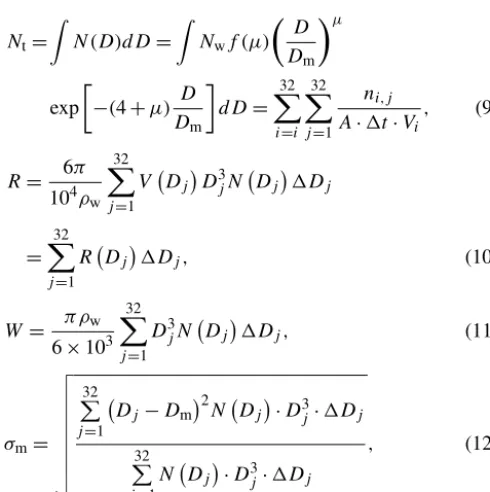
The integral parameters of total number concentra-tion Nt (m−3), rain rate R (mm h−1), liquid water
con-tent W (g m−3) and the mass spectrum standard devia-tionσm (mm) are also calculated in this study based on the
following equations. Nt=
Z
N (D)dD= Z
Nwf (µ)
D
Dm
µ
exp
−(4+µ) D Dm
dD=
32
X
i=i
32
X
j=1
ni,j
A·1t·Vi
, (9)
R= 6π 104ρw
32
X
j=1
V DjDj3N Dj1Dj
= 32
X
j=1
R Dj1Dj, (10)
W = π ρw 6×10³
32
X
j=1
Dj3N Dj
1Dj, (11)
σm=
v u u u u u u u t 32 P
j=1
Dj−Dm2N Dj
·Dj3·1Dj
32
P
j=1
N Dj·Dj3·1Dj
, (12)
where ρw is the water density (1.0 g cm−3);
R(Dj) (mm h−1mm−1) is the rain rate at the jth
di-ameter class, and it is normalized by the total rain rateRas R(Dj)norm=
R(Dj)
R in the analysis to resolve the
contribu-tion of different raindrop sizes to the rainfall intensities. The median volume diameterD0(mm) is defined such that drops
smaller than D0 contribute to half the total liquid water
content (W), as follows: π ρw
6×10³
D0 Z
0
D3N (D)dD=1 2
π ρw
6×10³, ∞
Z
0
D3N (D)dD=1
2(W ), (13)
is also computed and included in the analysis.
Considering that a high-resolution dual-polarization X-band radar network is being deployed in Beijing for ur-ban hydrometeorological applications, a series of polarimet-ric radar variables are simulated at X-band frequency based on the DSD measurements using theT-matrix method (Wa-terman, 1965; Leinonen, 2014), including horizontal reflec-tivityZH (mm6m−3), differential reflectivityZdr (dB), and
specific differential phase Kdp (◦km−1). The drop-shaped
model used in the simulation is the one proposed by Thurai et al. (2007). The temperature data are obtained from an au-tomatic weather station collocated with the THUD disdrom-eter. In addition, various DSD-based radar QPE relations are derived and their parameterization errors are investigated for future development of the Beijing urban radar rainfall sys-tem.
2.3 Quality control
To minimize the measurement errors and improve data reli-ability, several quality control procedures have been applied to the 1 min DSD data. First, because of the low signal-to-noise ratios, the lowest two diameter bins are not used. That is, the raindrops less than 0.312 mm are eliminated in the analysis. Second, the 1 min sample data with total raindrop number smaller than 10 or the derived rain rate less than 0.1 mm h−1are considered noise and are removed (Sreekanth et al., 2017). Then, if the continuous data satisfying the above conditions last less than 5 min, they will be ignored to avoid spurious and erratic measurements (Jash et al., 2019). In addition, to focus on rainfall, all the data contaminated by hail are removed, and raindrops at a diameter of larger than 8 mm are eliminated (Bringi and Chandrasekar, 2001) since the biggest raindrops ever reported globally in the literature are around 8 mm (Baumgardner and Colpitt, 1995; Beard et al., 1986). Also, thresholds on the simulated radar pa-rameters (i.e.,Zh=10log10ZH<55 dBZ, Zdr>0 dB, and
Kdp>0◦km−1) are implemented to further guarantee the
creditability of DSD data.
3 DSD parameter characteristics 3.1 Distribution of DSD parameters
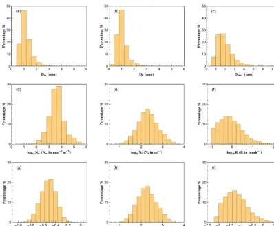
[image:4.612.46.291.268.514.2]A total number of 43 618 1 min DSD spectra have been se-lected after data quality control, covering the wet seasons (May to October) from 2014 to 2018 except for May 2014 (no observation then). In this study, the raindrops below 1 mm are considered small drops; 1–3 mm are midsize drops; and large drops if larger than 3 mm (Krishna et al., 2016; Seela et al., 2017, 2018; Tokay et al., 2014). The distri-bution and statistics of the DSD parameters are shown in Fig. 2 and Table 1.D0 andDm have similar distributions,
althoughD0has a larger range with a larger maximum and
Figure 2.Histograms of different DSD parameters for all selected rainfall:(a)mass-weighted mean diameter,Dm(mm);(b)median volume diameter,D0(mm);(c)maximum diameter,Dmax(mm);(d)generalized intercept parameter, log10Nw(Nwin m−3mm−1);(e)total number concentration, log10Nt(Ntin m−3);(f)rain rate, log10R(Rin mm h−1);(g)mass spectrum standard deviation, log10σm(σmin mm);(h)total number of raindrops, log10Td;(i)liquid water content, log10W(Win g m−3).
higher standard deviation, skewness and kurtosis values. The relationship3Dm+3.67=3D0+4 (Ulbrich, 1983) may be
explained for such a phenomenon when3 >0. The distribu-tion of Dmaxshows that during most of the rain events, the
biggest drops are the middle class size, indicating that most of the rainfall is potentially made up of small and moder-ate raindrops. The statistical characteristics of log10Nwshow
almost equal median (3.596) and mean values (3.595), as well as a very small skewness value (0.040), indicating that log10Nwfollows a symmetry distribution. The mean, median
and skewness values of log10Nt, log10Td, and log10σm also
exhibit symmetry distributions. Moreover, the kurtosis of these three parameters is close to 3, which indicates thatNt,
Td, andσmobey the lognormal distribution. Since a threshold
of 0.1 mm h−1is applied to the rain rate field (i.e., log10Ris truncated by −1), theR meets a positive skew distribution. Because of this, log10Walso has a positive skew distribution. It is worth noting that DSD samples with a rain rate about 0.8–1 mm h−1have the highest frequency and samples with a rain rate less than 1 mm h−1account for more than half of the total rain.
3.2 DSD properties for different rain types
Previous studies in different climate regions have shown that DSD may substantially differ in the two general pre-cipitation types (i.e., convective and stratiform), which has a great impact on the parameterization in both NWP mod-els and remote sensing observations. In this study, rainfall events are separated into stratiform and convective cases us-ing a method combinus-ing Brus-ingi et al. (2003) and Chen et al. (2013). In particular, if the standard derivation of rain rate for a consequent 10 min is greater than 1.5 mm h−1and the rain rate is greater than 5 mm h−1, it is classified as convec-tive rain; otherwise, it is classified as stratiform rain.
Figure 3 shows the histograms ofDmand log10Nwfor all
the rainfall events and for the convective and stratiform sub-sets. The three key statistics are also indicted in Fig. 3, in-cluding mean, standard deviation (SD), and skewness. For the total dataset (Fig. 3a), theDmhistogram is highly
posi-tively skewed, while the skewness of log10Nwis near to zero,
suggesting that the distribution of log10Nwis more
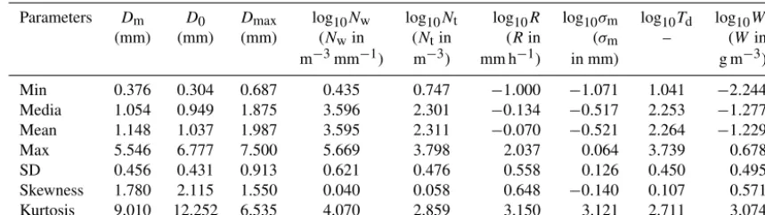
Table 1.Statistics of DSD parameters for all observations:Dm,D0,Dmax, log10Nw, log10Nt, log10R, log10σm, log10Tdand log10W.
Parameters Dm D0 Dmax log10Nw log10Nt log10R log10σm log10Td log10W
(mm) (mm) (mm) (Nwin (Ntin (Rin (σm – (Win
m−3mm−1) m−3) mm h−1) in mm) g m−3)
Min 0.376 0.304 0.687 0.435 0.747 −1.000 −1.071 1.041 −2.244
Media 1.054 0.949 1.875 3.596 2.301 −0.134 −0.517 2.253 −1.277
Mean 1.148 1.037 1.987 3.595 2.311 −0.070 −0.521 2.264 −1.229
Max 5.546 6.777 7.500 5.669 3.798 2.037 0.064 3.739 0.678
SD 0.456 0.431 0.913 0.621 0.476 0.558 0.126 0.450 0.495
Skewness 1.780 2.115 1.550 0.040 0.058 0.648 −0.140 0.107 0.571
Kurtosis 9.010 12.252 6.535 4.070 2.859 3.150 3.121 2.711 3.074
(0.46 mm forDm and 0.62 for log10Nw), indicating a high
variability of bothDmand log10Nw. The mean values ofDm
and log10Nware 1.15 mm and 3.60, respectively. It should be
noted that both mean values are slightly smaller compared with those obtained in the Beijing area during the summer time of 2015 (from 30 July to 30 September) and 2016 (from 9 June to 26 September) (G. Wen et al., 2017), which means that the DSD during summer time may be more concentrated than the whole rainy seasons.
Considering different rain types, it can be found that the Dmfor both types are positively skewed, while the skewness
of log10Nwfor convective is negative. The spread of log10Nw
for convective rain is narrower compared to that of strati-form rain, and the skewness of log10Nw is larger than that
of stratiform rain (−0.98 versus 0.10). The spreads and skewness of Dm for these two rainfall types perform
op-positely (see Fig. 3b and c). In addition, histograms ofDm
and log10Nwduring convective rain tend to shift toward the
large values relative to stratiform rain, indicating that convec-tive events have higherDmand log10Nw values than
strati-form cases (1.91 mm and 3.66 for convective versus 1.08 mm and 3.59 for stratiform, respectively).
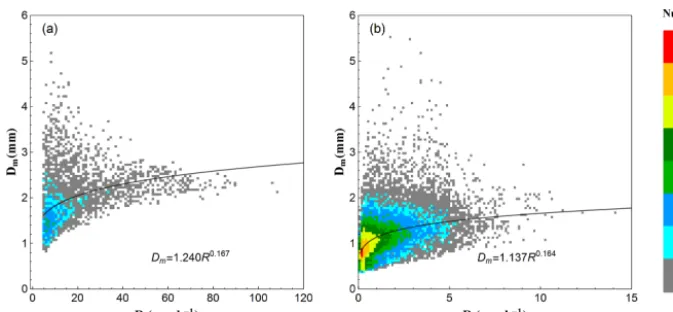
As Fig. 4 shows, in both convective and stratiform rains, with the increase in rain rate, the Dm increases (the
posi-tive exponents of the fitted power-law relationships), but the distributions ofDmbecome narrower. Note that at a higher
rain rate, the Dm values tend to be stable, indicating that
the DSD may have come to an equilibrium state where the coalescence and breakup of raindrops are in near balance (Hu and Srivastava, 1995). It can be seen in Fig. 4a that the Dm values reach a stable value around 2–2.5 mm when the
rain rateR >60 mm h−1, which means the increase in rain
rate is mainly caused by an increase in concentration (Bringi and Chandrasekar, 2001). With respect to the Dm–R
rela-tionship, the coefficient and exponent values of convective rain are slightly higher than stratiform, suggesting a larger Dm of convective rain than stratiform rain for a given rain
[image:6.612.309.550.229.569.2]rate, which is different from the findings in eastern China (Wen et al., 2016) or southern China (A. S. Zhang et al., 2019).
Figure 3.Histograms ofDmand log10Nw for(a)all the rainfall events,(b)convective events, and(c)stratiform events. Mean val-ues, standard deviation (SD), and skewness (SK) are also shown in the respective panels.
Figure 5 shows the distribution of log10NwversusDm
Figure 4.Scatter density plot forDm(mm) versusR(mm h−1) for(a)convective events and(b)stratiform events. The fitted power-law relationships are also provided in each panel adopting a least-squares method.
all the events combined, the distribution has a wide scale, but most points concentrate in the area of high log10Nwwith
low Dm. For convective and stratiform events, the
distri-butions are concentrated in different areas (stratiform: 3.3– 4.0 for log10Nw, 0.8–1.2 mm for Dm; convective: 3.7–4.2
for log10Nw, 1.4–2.0 mm for Dm). There is a rather clear
boundary between the two rainfall types, although there are some overlaps. For convective rain, there are more points in the “Continental cluster” than the “Maritime cluster”, but most points are neither in the “Continental cluster” nor in the “Maritime cluster” and have a tendency to approach the strat-iform rain. This indicates that the wet season convective rain in Beijing is neither maritime or continental as described by Bringi et al. (2003), which is likely due to the certain dis-tance between Beijing and the nearest ocean (about 160 km). For stratiform rainfall, the points are more concentrated, even with a wide range of log10NwversusDm. More than 85 % of
the stratiform points appear on the left side of the “strati-form line”. The average point of log10Nw−Dm for all the
rainfall events combined (magenta hollow star) also appears on the left side of the “stratiform line” due to the highest population of stratiform in the summer monsoon season (see also Table 2). These indicate the lower diameter and higher concentration characteristics of rainfall in the Beijing area. The relationship of log10Nw−D0 (see Fig. S1 in the
Sup-plement) shows that the line to classify rain types based on log10Nw−D0(Thurai et al., 2016) would misclassify more
convective rain as stratiform rain. This is probably due to the complex terrain in Beijing (Fig. 1a), where the high moun-tain to the west may have a substantial impact on the rain evolving from the western mainland.
The comparison of DSDs in different parts of China shows interesting results. Even in the same region, the DSDs measured by different instruments have notable dif-ferences, such as the differences in Beijing between re-sults from G. Wen et al. (2017) (2DVD, circle) and Tang et al. (2014) (Parsivel, square). In order to reduce the
er-rors caused by different measurement instruments, only DSDs measured by Parsivel disdrometers are analyzed in this study. It is concluded that the eastern part of China has the lowest mean value of log10Nw (3.42) and highest
mean value of Dm (1.66), while southern China has the
highest mean value of log10Nw (3.86) with a middle value
ofDm(1.46), and the northern part of China has the middle
value of log10Nw (3.60) with a lowest value of Dm (1.15).
This highlights that the DSD characteristics are highly de-pendent on the specific geographical locations and associated climate regimes. The results of Beijing from this study and Tang et al. (2014) show great differences in convective rain and lesser differences in stratiform rain, which is attributed to different convective systems during different years.
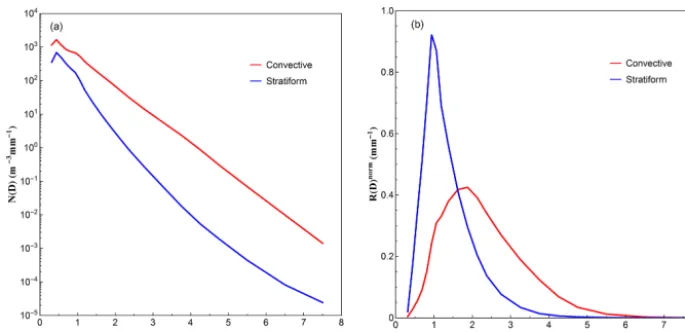
The DSD spectra andR(D)distributions of two rain types are shown in Fig. 6. Substantial differences are observed between these two rainfall types in both DSD spectra and R(D)distributions. The peaks of DSD spectra for both rain-fall types are at the same diameter bin aroundD∼0.5 mm, while the spectrum for convective is higher than that of strat-iform. The peak ofR(D)distribution for stratiform rain is at the diameter around 0.9 mm and 1.9 mm for convective rain, which is much larger than where the DSD spectra peaks occur due to theD3dependency ofR(D). In addition, the distribution ofR(D)for convective rain is much lower and broader. The differences in DSD spectra andR(D) distribu-tions indicate that the convective rainfall has a higher concen-tration of moderate- to large-sized drops, and the large drops contribute more to convective rainfall compared to stratiform rainfall.
3.3 DSD characteristics in different rain rate classes
Figure 5.Scatter density plot of log10Nw versusDm:(a)the total rainfall events;(c)stratiform events;(d)convective events.(b)is the scatterplot of log10NwversusDmfor the convective (red circle dots) and stratiform (blue square dots) cases. The two black rectangles in each subplot correspond to the maritime and continental convective clusters, and the black dashed line is the log10Nw–Dmrelationship for stratiform rain reported by Bringi et al. (2003). The cross, hollow triangles, circle, squares, diamonds, and hearts in(b)represent the averaged values obtained in previous studies by Chen et al. (2013), Wen et al. (2016), G. Wen et al. (2017), Tang et al. (2014), and A. S. Zhang et al. (2019) for different parts of China. The colors of these symbols represent different events: magenta for total rainfall events; green for convective events; yellow for stratiform events; and black for the shallow events, a third type of precipitation besides convective and stratiform suggested by a few researchers, based on data from vertically pointing radar observations (Fabry and Zawadzki, 1995; Cha et al., 2009) in the study by Wen et al. (2016).
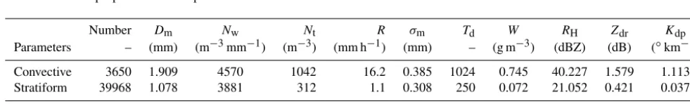
Table 2.Statistical properties of DSD parameters for convective and stratiform rain.
Number Dm Nw Nt R σm Td W RH Zdr Kdp
Parameters – (mm) (m−3mm−1) (m−3) (mm h−1) (mm) – (g m−3) (dBZ) (dB) (◦km−1)
Convective 3650 1.909 4570 1042 16.2 0.385 1024 0.745 40.227 1.579 1.113
Stratiform 39968 1.078 3881 312 1.1 0.308 250 0.072 21.052 0.421 0.037
Total 43618 1.148 3938 373 2.4 0.314 315 0.128 22.656 0.518 0.128
1≤R <2; C4, 2≤R <5; C5, 5≤R <10; C6, 10≤R < 25; C7, 25≤R <50; C8,R≥50 mm h−1. Such classifica-tion is based on the fact of high frequency of low rain rates in the Beijing area as well as several previous studies, including Das and Maitra (2016), Harikumar et al. (2010), Krishna et al. (2016), Sarkar et al. (2015), and Tokay and Short (1996). The DSD sample numbers and rain rate statistics for each cat-egory are summarized in Table 3. For each rain rate class, the
[image:8.612.52.543.529.603.2]Figure 6.Composite raindrop spectra(a)and normalizedR(D)distributions(b)for different rain types.
Figure 7.Same as Fig. 6 but for different rain rate classes.
al., 2012). All the DSD spectra only have one peak, which differs from Krishna et al. (2016), where the spectrum be-comes bimodal when the rain rate R >8 mm h−1. In addi-tion, the peaks of all DSD spectra are at a diameter around D∼0.5 mm, which is different from Jash et al. (2019) for In-dia, where the peak position shifts towards larger diameters as the rain rate increases.
The mean normalized R(D) of each rain rate class is shown in Fig. 7b, illustrating the contribution of each diam-eter bin to the total rainwater. The normalized rain rate dis-tributions are unimodal and the peaks are around D∼0.9– 2.5 mm. The peak position shifts to a larger diameter and the distribution becomes lower and broader as rain rate increases. These results are similar to those in Jash et al. (2019) for In-dia but different from those in Peters et al. (2002) for Ger-many, where theR(D)distribution has a secondary peak at lower rain rate intensity (R <1 mm h−1). This analysis im-plies that raindrops of diameter 0.9–2.5 mm (i.e., moderate
size) contribute most towards accumulated rainwater during the rainy season in the Beijing area, and the size of drops contributing the most rainfall increases as the rainfall inten-sity increases.
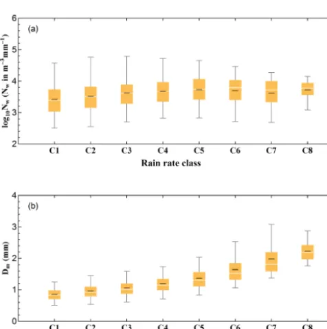
Variations of the normalized intercept parame-ter (log10Nw) and mass-weighted mean diameter (Dm)
in each rain rate class are provided in Fig. 8 with a box-whisker plot. It can be seen thatDmvalues increase with the
increase in rainfall intensity, while the increasing trend of log10Nw is not as clear. This could be due to the imbalance
between the decrease in small drop concentration and the increase in midsize and large drop concentration at a higher rain rate (R >10 mm h−1, from C6 to C8). The means and standard deviations ofDm, log10Nw, Nt,W,µ, and3 for
each rain rate class are provided in Table 4, which clearly shows that with the increase in rainfall intensity, the mean values of total number concentration (Nt)and liquid water
[image:9.612.101.498.266.463.2]Table 3.Number and DSD retrieved rain rate statistics of each rain rate class.
Rain rate No. of Mean SD Skewness Kurtosis
threshold samples mm h−1 mm h−1
C1 0.1≤R <0.5 16 464 0.27 0.11 0.36 1.96
C2 0.5≤R <1 9340 0.72 0.14 0.29 1.92
C3 1≤R <2 7466 1.43 0.29 0.29 1.90
C4 2≤R <5 6145 3.08 0.82 0.62 2.26
C5 5≤R <10 2141 6.93 1.41 0.47 2.06
C6 10≤R <25 1463 15.47 4.11 0.58 2.25
C7 25≤R <50 446 34.85 6.91 0.42 1.96
[image:10.612.51.289.228.467.2]C8 R≥50 153 62.98 10.95 1.39 5.44
Figure 8. Variation of the normalized intercept parameter log10Nw(a)and the mass-weighted mean diameterDm(b)for dif-ferent rain rate classes. The white central line of the box indicates the median, the black central line in the box indicates the mean val-ues, and the bottom and top lines of the box indicate the 25th and 75th percentiles, respectively. The bottom and top lines of the ver-tical lines out of the box indicate the 5th and 95th percentiles, re-spectively.
parameter (µ)and slope parameter (3) show a decreasing trend, resulting in a wider breadth and lower peak of DSD at high rain rates.
3.4 Diurnal variations of DSD characteristics
Since the 1980s, Beijing has been experiencing rapid urban-ization, causing a lot of problems, among which UHI is one of the most well-known phenomena (Yang et al., 2013b). Some studies showed that extreme precipitation events are more likely to occur during the period when the UHI
inten-sity is high, usually from late afternoon to early morning in Beijing local time (LST) (Li et al., 2008; Song et al., 2014; Yang et al., 2013a, 2017; Y. Y. Zhang et al., 2019). In or-der to explore the DSD variations during the day, the di-urnal periods are divided into four parts based on the UHI variation described in Yang et al. (2013b): strong UHI stage (S UHI, 21:00–06:00 LST), weak UHI stage (W UHI, 11:00– 16:00 LST), UHI down stage characterized by a fast de-cline of UHI intensity (UHI D, 06:00–11:00 LST) and UHI up stage characterized by an abrupt rise of UHI intensity (UHI U, 16:00–21:00 LST). The rain rate and DSD charac-teristics corresponding to these four stages are shown in Ta-ble 5. The DSD spectra andR(D)distributions are shown in Fig. 9.
Figure 9.Same as Fig. 6 but for different diurnal periods based on UHI intensity.
plots of variation ofDmand log10Nwfor each diurnal period
show the same results (see Fig. 10). The W UHI stage has the highest mean concentration and the lowest meanDmvalue,
while the UHI U stage has the largest meanDmvalue and the
S UHI stage has the lowest mean concentration. 3.5 DSD characteristics in different months
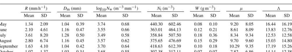
To obtain a better understanding of the seasonal variations of DSD characteristics in the Beijing urban area, rain data collected in different months are analyzed. The rain rate and DSD characteristics for different months are shown in Ta-ble 6. Figure 11 illustrates the corresponding DSD spectra andR(D)distributions.
As shown in Fig. 11, all the DSD spectra have peaks at di-ameterD∼0.5 mm, which are consistent with other classifi-cations in this study. The DSD in May has a relatively higher concentration and a relatively lower concentration in July. At small drop size bins (D <1 mm), the spectra for May and September are similar, while the spectra for the other 4 months are similar. As the diameter increases, the differences between these spectra become larger, and the DSD spectrum for July has the highest concentration and October the low-est concentration. The rainfall with higher concentration and
large drops is more likely to happen in July, leading to a high rain rate intensity (see also Fig. S3).
It is also noted that theR(D)distributions for each month are different from each other. The distributions of May, Oc-tober, and September have a peak at diameter aroundD∼ 0.9 mm, while the distributions of June and August have a peak at diameter around D∼1 mm. TheR(D) distribu-tion of July has two peaks at diameter around D∼1 and D∼1.5 mm. In addition, the R(D) distribution of July is the widest and lowest, suggesting that a wide range of moderate drops contribute mostly to the rain in July. The Dmand log10Nw in Fig. 12 show an interesting annual
cy-cle: the Dm (log10Nw) first goes up and (down) then goes
down (up), while in JulyDm(log10Nw) reaches the highest
(lowest) value.
4 Implications for radar rainfall estimation 4.1 Single polarized radar applications
[image:11.612.47.548.78.391.2]How-Table 5.Mean and standard deviation (SD) values ofR,Dm, log10Nw,Nt,W,µ, and3for different diurnal periods based on UHI intensity.
R(mm h−1) Dm(mm) log10Nw(m−3mm−1) Nt(m−3) W(g m−3) µ 3
Mean SD Mean SD Mean SD Mean SD Mean SD Mean SD Mean SD
[image:12.612.47.552.84.156.2]UHI D 1.88 4.31 1.11 0.42 3.59 0.60 342.15 499.30 0.10 0.19 15.06 13.63 9.32 8.49 W UHI 2.04 4.10 1.10 0.41 3.70 0.58 378.44 398.08 0.12 0.18 15.27 14.48 9.33 8.90 UHI U 2.82 6.94 1.18 0.51 3.57 0.65 380.88 488.27 0.15 0.30 14.09 13.45 8.78 8.45 S UHI 2.60 6.79 1.18 0.46 3.56 0.64 385.00 563.30 0.14 0.30 13.97 13.95 8.61 8.43
Table 6.Mean and standard deviation (SD) values ofR,Dm, log10Nw,Nt,W,µ, and3for each month.
R(mm h−1) Dm(mm) log10Nw(m−3mm−1) Nt(m−3) W(g m−3) µ 3
Mean SD Mean SD Mean SD Mean SD Mean SD Mean SD Mean SD
May 1.34 2.09 1.04 0.39 3.74 0.68 440.30 602.46 0.08 0.10 9.20 8.05 16.44 16.19
June 2.10 4.61 1.16 0.47 3.55 0.66 363.01 464.13 0.12 0.21 8.61 8.09 13.83 12.76
July 3.61 8.20 1.28 0.50 3.49 0.58 358.84 507.50 0.18 0.36 8.34 9.34 12.53 12.58
August 2.80 6.74 1.16 0.45 3.57 0.62 375.65 476.69 0.15 0.29 9.70 9.60 15.03 14.80 September 1.63 4.10 1.04 0.42 3.70 0.64 418.63 612.39 0.10 0.18 10.29 9.35 17.19 15.26 October 1.07 1.37 1.03 0.34 3.68 0.55 307.38 312.11 0.07 0.07 7.82 6.86 14.14 12.38
Figure 10.Same as Fig. 8 but for different diurnal periods based on UHI intensity.
ever, the coefficient a and exponent b greatly rely on the DSD variability (Bringi et al., 2003; Rosenfeld and Ul-brich, 2003; Uijlenhoet, 2001). The default Z–R relation-ship applied for the operational Weather Surveillance Radar – 1988 Doppler (WSR-88D) systems in the United States isZ=300R1.4(Fulton et al., 1998), whereasZ=200R1.6 is commonly used in the continental area for stratiform rain (Marshall and Palmer, 1948, hereafter referred to as the MP-Stratiform relationship). The more appropriate and local-izedaandb are expected to improve regional radar rainfall
estimation. In the following, the localizedZ–Rrelationships for different rain types are derived by the nonlinear least-squares method, aiming to provide references for operational S-band radar rainfall applications in Beijing.
Figure 13 shows the scatter density plot of rain rate ver-sus horizontal reflectivity, as well as the fitted power-law re-lations for different rain types. Figure 13 shows that most of the samples are at low values where bothZH andR are
small, which also suggests that the DSD may be under size-controlled conditions (Steiner et al., 2004). Meanwhile, the relationship for total rainfall (Z=238R1.57) underestimates the rain rate at low values compared with the stratiform re-lationship (Z=171R2.15), due to the inconsistent rain rate– reflectivity structures of two rain types.
The default NEXRAD algorithm and MP-Stratiform re-lationship for continental stratiform rain are also indicated in Fig. 13 for comparison. At low reflectivity values (ZH<
23 dBZ), the curve of the MP-Stratiform relationship is be-low the local stratiform relation, but at higher values, it re-verses. As the mean reflectivity of stratiform rain (21 dBZ) is less than 23 dBZ (see Table 2), the MP-Stratiform relation-ship may introduce underestimation of rainfall. The default NEXRAD relationship behaves similarly: underestimation at lower reflectivity values and overestimation at higher reflec-tivity values. Considering the mean reflecreflec-tivity value of con-vective rain, the default NEXRAD relationship may cause overestimation of rainfall. In other words, the default rela-tionshipZ=300R1.4should be used with caution for local applications in Beijing.
4.2 High-frequency (X-band) polarimetric radar applications
[image:12.612.56.557.192.281.2] [image:12.612.48.289.251.538.2]Figure 11.Same as Fig. 6 but for different months.
Figure 12.Same as Fig. 8 but for different months.
in the Beijing area. To support the radar deployment and facilitate the rainfall applications, the polarimetric parame-ters, including differential reflectivityZdr (dB) and specific
differential propagation-phase shift Kdp (◦km−1), are
com-puted from the DSD measurements. Therein, the T-matrix method (Waterman, 1965) is adopted and the computations are made at X-band frequency. In addition, the polarimet-ric rainfall relations are derived based on the nonlinear least-squares method, includingR(Kdp),R(Kdp,ZDR), andR(ZH,
ZDR). HereZDR=10Zdr/10is the differential reflectivity in
the linear scale.
Figure 13. Scatter density plot of R (mm h−1) ver-sus ZH (mm6m−3) for all rain events. The black, red, and blue curves, respectively, stand for the fitted power-law relations for total rain, convective rain, and stratiform rain. The purple and green dashed lines denote the default NEXRAD Z–R relation (Fulton et al., 1998) and a commonly used continental stratiform rain relation (Marshall and Palmer, 1948), respectively.
The derived X-band radar rainfall relations are as follows:
R (ZH)=0.0576ZH0.557, (14)
R Kdp
=15.421Kdp0.817, (15)
R Kdp, ZDR
=26.778Kdp0.946ZDR−1.249, (16) R (ZH, ZDR)=5.886×10⁻³ZH0.994Z
−4.929
DR . (17)
Figure 14.Scatter density plots of rainfall rates estimated from radar rainfall relations versus rain rates calculated directly from DSD: (a)R(ZH),(b)R(Kdp),(c)(Kdp,ZDR), and(d)R(ZH,ZDR). The black diagonal line in each panel represents the 1–1 relationship.
among the key factors affecting the derived rainfall perfor-mance (Bringi and Chandrasekar, 2001). Hence, the param-eterization errors in the X-band radar rainfall algorithms are investigated and quantified in this study. Figure 14 illustrates the scatter density plots of rain rates derived from R(ZH),
R(Kdp),R(Kdp,ZDR), andR(ZH,ZDR)versus the rain rates
directly computed from DSD. To quantify the parameteriza-tion errors, the normalized mean absolute error (NMAE) of the estimated rainfall rate is calculated, which is defined as NMAE=h|REP−RD|i
hRDi
, (18)
where the angle brackets stand for sample average;REPand
RD denote the estimated rain rates derived from
parameter-ized radar rainfall algorithms and DSD information, respec-tively. The NMAERR is calculated for different rainfall rate
intervals from 0 to 100 mm h−1. Figure 15 shows the
param-eterization error structure ofR(ZH),R(Kdp),R(Kdp,ZDR),
andR(ZH,ZDR)as a function of rainfall rate.
It can be seen from Figs. 14 and 15 that the algo-rithms based on dual-polarization radar parameters can pro-vide better estimates than theZ–Rrelationship. In addition, the dual-parameter algorithms, namely R(Kdp, ZDR) and
R(ZH,ZDR), have even better performance than the
single-parameter-based algorithm including R(Kdp). The NMAE
has a decreasing trend as the rain rate increases from 1 to 60 mm h−1. The fluctuation when rain rate is greater than 60 mm h−1 may be due to the random errors caused by a few samples of large values. The parameterization errors of R(Kdp),R(Kdp,ZDR), andR(ZH,ZDR)become stable when
rain rate becomes higher than 10 mm h−1. It is also noted that at low rain rate (less than 10 mm h−1), the NMAE ofR(ZH,
ZDR)is the smallest, while at higher rain rate (higher than
10 mm h−1) the NMAE ofR(Kdp,ZDR)becomes the
small-est. This again highlights the importance of selecting appro-priate rain rate relations for local radar applications.
5 Summary and conclusion
In this paper, 5-year (2014–2018) observations of DSD from a disdrometer deployed at Tsinghua University are analyzed to explore the microphysical characteristics of precipitation during rainy seasons (May–October) in the Beijing urban area. The main conclusions are as follows.
1. For all rain events, all the DSD parameters (Dm,D0,
Dmax, log10Nw, log10Nt, log10R, log10σm, log10Tdand
Figure 15.Parameterization error structure ofR(ZH),R(Kdp),R(Kdp,ZDR), andR(ZH,ZDR)as a function of rainfall rate:(a)for mean rain rate less than 10 mm h−1;(b)for rain rate of the whole dataset.
a high frequency of low values and a low frequency of high values in the Beijing urban area. More than half of the DSD measurements are characterized by a rainfall rate of less than 1 mm h−1.
2. The mean values of log10Nw and Dm of convective
rain are higher than that of stratiform rain, indicating a higher raindrop concentration and larger drop size dur-ing convective events. This is also in line with the rain-drop spectra and normalized R(D)distribution. In ad-dition, log10Nwof convective rain is negatively skewed,
which is opposite to that of stratiform rain. For both rainfall types, theDm values are higher but the
distri-butions are narrower at higher rainfall intensities. 3. There is a clear boundary to distinguish between
convective and stratiform rain from the scatterplot of log10Nw versus Dm. However, the convective rain
in the Beijing area is neither continental nor maritime as described by Bringi et al. (2003), due to the partic-ular location and complex topography. Moreover, the comparison with different parts of China shows that the DSD variability is closely related to geographic loca-tion, climate regimes and study periods.
4. Stratified by rain rate, the DSD spectra become higher and wider as the rain rate increases, but all have peaks at the similar diameter sizeD∼0.5 mm. The peaks of the normalizedR(D)distribution shift to larger diame-ter size (still within the midsize range) and the distribu-tion becomes lower and wider as the rain rate increases. Meanwhile, the Dm and log10Nw show an increasing
trend and the slope parameter (µ) shows a decreasing trend as the rain rate increases.
5. During the periods of strong UHI and UHI up stages, the DSD spectra trend to have a higher concentration
at large size drops and largerDmvalues than other
pe-riods, indicating intense rainfall during these periods. The DSD has similar characteristics in July and August. In addition, theDmand log10Nwvalues show a diurnal
cycle and an annual cycle. All these findings indicate substantial temporal variabilities of DSD in Beijing. 6. TheZ–R relationship derived from local DSD in
Bei-jing is quite different from the operational NEXRAD al-gorithm (MP-Stratiform) which may overestimate (un-derestimate) rainfall at high (low) rain intensity. The er-ror structures of different algorithms show that the po-larimetric radar rainfall relationsR(Kdp),R(Kdp,ZDR),
andR(ZH,ZDR)have greater potential thanZ–R
meth-ods for urban QPE.
Data availability. Disdrometer data used in this study are available by contacting the authors.
Supplement. The supplement related to this article is available on-line at: https://doi.org/10.5194/hess-23-4153-2019-supplement.
Author contributions. YM, GN, FT and HC conceived the idea; GN and FT provided financial support and observation data; YM conducted the detailed analysis; HC and CVC provided com-ments on the analysis; all the authors contributed to the writing and revisions.
Competing interests. The authors declare that they have no conflict of interest.
Acknowledgements. This research was supported by the Ministry of Science and Technology of the People’s Republic of China un-der grant 2013DFG72270 and the National Key Research and De-velopment Program of China under grant 2018YFA0606002. Yu Ma was also supported by the China Scholarship Council and Ts-inghua University Tutor Research Fund. Participation of Chan-drasekar V. Chandra and Haonan Chen was also supported by the US National Science Foundation Hazards SEES program and the California Department of Water Resources, respectively.
Financial support. This research has been supported by the Min-istry of Science and Technology of the People’s Republic of China (grant no. 2013DFG72270) and the National Key Research and De-velopment Program of China (grant no. 2018YFA0606002).
Review statement. This paper was edited by Xing Yuan and re-viewed by Long Yang and one anonymous referee.
References
Abel, S. J. and Boutle, I. A.: An improved representation of the raindrop size distribution for single-moment micro-physics schemes, Q. J. Roy. Meteorol. Soc., 138, 2151–2162, https://doi.org/10.1002/qj.1949, 2012.
Angulo-Martinez, M. and Barros, A. P.: Measurement uncertainty in rainfall kinetic energy and intensity relationships for soil ero-sion studies: An evaluation using PARSIVEL disdrometers in the Southern Appalachian Mountains, Geomorphology, 228, 28–40, https://doi.org/10.1016/j.geomorph.2014.07.036, 2015. Atlas, D., Srivastava, R. C., and Sekhon, R. S.: Doppler Radar
Char-acteristics of Precipitation at Vertical Incidence, Rev. Geophys., 11, 1–35, https://doi.org/10.1029/RG011i001p00001, 1973. Battan, L. J.: Radar observation of the atmosphere, University of
Chicago Press, Chicago, 324 pp., 1973.
Baumgardner, D. C. and Colpitt, A.: Monster drops and rain gushes: unusual precipitation phenomena in Florida marine cumulus, in:
Proc. Conf. Cloud Physics, January 1995, Boston, USA, 15–20, 1995.
Beard, K. V., Johnson, D. B., and Baumgardner, D.: Air-craft Observations of Large Raindrops in Warm, Shal-low, Convective Clouds, Geophys. Res. Lett., 13, 991–994, https://doi.org/10.1029/GL013i010p00991, 1986.
Bringi, V. N. and Chandrasekar, V.: Polarimetric Doppler weather radar: principles and applications, Cambridge University Press, Cambrigde, 2001.
Bringi, V. N., Chandrasekar, V., Hubbert, J., Gorgucci, E., Randeu, W. L., and Schoenhuber, M.: Raindrop size distribution in different climatic regimes from disdrometer and dual-polarized radar analysis, J. At-mos. Sci., 60, 354–365, https://doi.org/10.1175/1520-0469(2003)060<0354:Rsdidc>2.0.Co;2, 2003.
Caracciolo, C., Napoli, M., Porcù, F., Prodi, F., Dietrich, S., Zanchi, C., and Orlandini, S.: Raindrop size distribu-tion and soil erosion, J. Irrig. Drain. Eng., 138, 461–469, https://doi.org/10.1061/%28ASCE%29IR.1943-4774.0000412, 2011.
Cha, J.-W., Chang, K.-H., Yum, S. S., and Choi, Y.-J.: Compari-son of the bright band characteristics measured by Micro Rain Radar (MRR) at a mountain and a coastal site in South Korea, Adv. Atmos. Sci., 26, 211–221, 2009.
Chen, B. J., Yang, J., and Pu, J. P.: Statistical Characteris-tics of Raindrop Size Distribution in the Meiyu Season Ob-served in Eastern China, J. Meteorol. Soc. Jpn., 91, 215–227, https://doi.org/10.2151/jmsj.2013-208, 2013.
Chen, H. and Chandrasekar, V.: The quantitative precipita-tion estimaprecipita-tion system for Dallas–Fort Worth (DFW) ur-ban remote sensing network, J. Hydrol., 531, 259–271, https://doi.org/10.1016/j.jhydrol.2015.05.040, 2015.
Cifelli, R., Chandrasekar, V., Chen, H. N., and Johnson, L. E.: High Resolution Radar Quantitative Precipitation Estimation in the San Francisco Bay Area: Rainfall Monitoring for the Urban Environment, J. Meteorol. Soc. Jpn., 96a, 141–155, https://doi.org/10.2151/jmsj.2018-016, 2018.
Cristiano, E., ten Veldhuis, M.-C., and van de Giesen, N.: Spatial and temporal variability of rainfall and their effects on hydro-logical response in urban areas – a review, Hydrol. Earth Syst. Sci., 21, 3859–3878, https://doi.org/10.5194/hess-21-3859-2017, 2017.
Das, S. and Maitra, A.: Vertical profile of rain: Ka band radar observations at tropical locations, J. Hydrol., 534, 31–41, https://doi.org/10.1016/j.jhydrol.2015.12.053, 2016.
Deo, A. and Walsh, K. J. E.: Contrasting tropical cyclone and non-tropical cyclone related rainfall drop size dis-tribution at Darwin, Australia, Atmos. Res., 181, 81–94, https://doi.org/10.1016/j.atmosres.2016.06.015, 2016.
de Vos, L., Leijnse, H., Overeem, A., and Uijlenhoet, R.: The po-tential of urban rainfall monitoring with crowdsourced automatic weather stations in Amsterdam, Hydrol. Earth Syst. Sci., 21, 765–777, https://doi.org/10.5194/hess-21-765-2017, 2017. Dolan, B., Fuchs, B., Rutledge, S. A., Barnes, E. A., and
Harikumar, R., Sampath, S., and Kumar, V. S.: Variation of rain drop size distribution with rain rate at a few coastal and high altitude stations in southern peninsular India, Adv. Space Res., 45, 576– 586, https://doi.org/10.1016/j.asr.2009.09.018, 2010.
Hou, A. Y., Kakar, R. K., Neeck, S., Azarbarzin, A. A., Kummerow, C. D., Kojima, M., Oki, R., Nakamura, K., and Iguchi, T.: The Global Precipitation Measurement Mission, B. Am. Meteorol. Soc., 95, 701–722, https://doi.org/10.1175/Bams-D-13-00164.1, 2014.
Hu, Z. L. and Srivastava, R. C.: Evolution of Rain-drop Size Distribution by Coalescence, Breakup, and Evaporation – Theory and Observations, J. Atmos. Sci., 52, 1761–1783, https://doi.org/10.1175/1520-0469(1995)052<1761:Eorsdb>2.0.Co;2, 1995.
Iguchi, T., Kozu, T., Meneghini, R., Awaka, J., and Okamoto, K.: Rain-profiling algorithm for the TRMM precipitation radar, J. Appl. Meteorol., 39, 2038–2052, https://doi.org/10.1175/1520-0450(2001)040<2038:Rpaftt>2.0.Co;2, 2000.
Islam, T., Rico-Ramirez, M. A., Thurai, M., and Han, D.: Charac-teristics of raindrop spectra as normalized gamma distribution from a Joss–Waldvogel disdrometer, Atmos. Res., 108, 57-73, 10.1016/j.atmosres.2012.01.013, 2012.
Jash, D., Resmi, E. A., Unnikrishnan, C. K., Sumesh, R. K., Sreekanth, T. S., Sukumar, N., and Ramachandran, K. K.: Vari-ation in rain drop size distribution and rain integral parameters during southwest monsoon over a tropical station: An inter-comparison of disdrometer and Micro Rain Radar, Atmos. Res., 217, 24–36, https://doi.org/10.1016/j.atmosres.2018.10.014, 2019.
Ji, L., Chen, H., Li, L., Chen, B., Xiao, X., Chen, M., and Zhang, G. J. R. S.: Raindrop Size Distributions and Rain Characteristics Observed by a PARSIVEL Disdrome-ter in Beijing, Northern China, Remote Sens., 11, 1479, https://doi.org/10.3390/rs11121479, 2019.
Kinnell, P. I. A.: Raindrop-impact-induced erosion processes and prediction: a review, Hydrol. Process., 19, 2815–2844, https://doi.org/10.1002/hyp.5788, 2005.
Kozu, T. and Nakamura, K.: Rainfall Parameter-Estimation from Dual-Radar Measurements Combining Reflectiv-ity Profile and Path-Integrated Attenuation, J. Atmos. Ocean. Tech., 8, 259–270, https://doi.org/10.1175/1520-0426(1991)008<0259:Rpefdr>2.0.Co;2, 1991.
Krishna, U. V. M., Reddy, K. K., Seela, B. K., Shirooka, R., Lin, P. L., and Pan, C. J.: Raindrop size distribution of east-erly and westeast-erly monsoon precipitation observed over Palau
is-Ocean. Tech., 17, 130–139, https://doi.org/10.1175/1520-0426(2000)017<0130:Aodfms>2.0.Co;2, 2000.
Lyu, H., Ni, G. H., Cao, X. J., Ma, Y., and Tian, F. Q.: Effect of Temporal Resolution of Rainfall on Simulation of Urban Flood Processes, Water, 10, 880, https://doi.org/10.3390/w10070880, 2018.
Marshall, J. S. and Palmer, W. M.: The
Dis-tribution of Raindrops with Size, J. Meteo-rol., 5, 165–166, https://doi.org/10.1175/1520-0469(1948)005<0165:Tdorws>2.0.Co;2, 1948.
McFarquhar, G. M., Hsieh, T.-L., Freer, M., Mascio, J., and Jew-ett, B. F.: The Characterization of Ice Hydrometeor Gamma Size Distributions as Volumes inN0–λ–µPhase Space: Implications for Microphysical Process Modeling, J. Atmos. Sci., 72, 892– 909, https://doi.org/10.1175/jas-d-14-0011.1, 2015.
Montopoli, M., Marzano, F. S., and Vulpiani, G.: Analysis and synthesis of raindrop size distribution time series from disdrometer data, IEEE T. Geosci. Remote, 46, 466–478, https://doi.org/10.1109/Tgrs.2007.909102, 2008.
Peters, G., Fischer, B., and Andersson, T.: Rain observations with a vertically looking Micro Rain Radar (MRR), Boreal Environ. Res., 7, 353–362, 2002.
Rosenfeld, D. and Ulbrich, C. W.: Cloud microphysical prop-erties, processes, and rainfall estimation opportunities, in: Radar and Atmospheric Science: A Collection of Essays in Honor of David Atlas, American Meteorological So-ciety, Boston, MA, 237–258, https://doi.org/10.1175/0065-9401(2003)030<0237:CMPPAR>2.0.CO;2, 2003.
Saleeby, S. M. and Cotton, W. R.: A large-droplet mode and prognostic number concentration of cloud droplets in the Colorado State University Regional Atmo-spheric Modeling System (RAMS). Part I: Module descriptions and supercell test simulations, J. Appl. Meteorol., 43, 182–195, https://doi.org/10.1175/1520-0450(2004)043<0182:Almapn>2.0.Co;2, 2004.
Sarkar, T., Das, S., and Maitra, A.: Assessment of different rain-drop size measuring techniques: Inter-comparison of Doppler radar, impact and optical disdrometer, Atmos. Res., 160, 15–27, https://doi.org/10.1016/j.atmosres.2015.03.001, 2015.
Seela, B. K., Janapati, J., Lin, P. L., Wang, P. K., and Lee, M. T.: Raindrop Size Distribution Characteris-tics of Summer and Winter Season Rainfall Over North Taiwan, J. Geophys. Res.-Atmos., 123, 11602–11624, https://doi.org/10.1029/2018jd028307, 2018.
Smith, J. A., Hui, E., Steiner, M., Baeck, M. L., Krajewski, W. F., and Ntelekos, A. A.: Variability of rainfall rate and raindrop size distributions in heavy rain, Water Resour. Res., 45, W04430, https://doi.org/10.1029/2008wr006840, 2009.
Song, X. M., Zhang, J. Y., AghaKouchak, A., Sen Roy, S., Xuan, Y. Q., Wang, G. Q., He, R. M., Wang, X. J., and Liu, C. S.: Rapid urbanization and changes in spatiotemporal characteristics of precipitation in Beijing metropolitan area, J. Geophys. Res.-Atmos., 119, 11250–11271, https://doi.org/10.1002/2014jd022084, 2014.
Sreekanth, T. S., Varikoden, H., Sukumar, N., and Kumar, G. M.: Microphysical characteristics of rainfall during different seasons over a coastal tropical station using disdrometer, Hydrol. Pro-cess., 31, 2556–2565, https://doi.org/10.1002/hyp.11202, 2017. Steiner, M., Smith, J. A., and Uijlenhoet, R.: A
microphysi-cal interpretation of radar reflectivity–rain rate relationships, J. Atmos. Sci., 61, 1114–1131, https://doi.org/10.1175/1520-0469(2004)061<1114:AMIORR>2.0.CO;2, 2004.
Tang, Q., Xiao, H., Guo, C. W., and Feng, L.: Characteristics of the raindrop size distributions and their retrieved polarimetric radar parameters in northern and southern China, Atmos. Res., 135, 59–75, https://doi.org/10.1016/j.atmosres.2013.08.003, 2014. Testud, J., Le Bouar, E., Obligis, E., and Ali-Mehenni, M.: The rain
profiling algorithm applied to polarimetric weather radar, J. At-mos. Ocean. Tech., 17, 332–356, https://doi.org/10.1175/1520-0426(2000)017<0332:TRPAAT>2.0.CO;2, 2000.
Thurai, M., Huang, G. J., Bringi, V. N., Randeu, W. L., and Schön-huber, M.: Drop Shapes, Model Comparisons, and Calculations of Polarimetric Radar Parameters in Rain, J. Atmos. Ocean. Tech., 24, 1019–1032, https://doi.org/10.1175/jtech2051.1, 2007.
Thurai, M., Gatlin, P. N., and Bringi, V. N.: Separating stratiform and convective rain types based on the drop size distribution char-acteristics using 2D video disdrometer data, Atmos. Res., 169, 416–423, https://doi.org/10.1016/j.atmosres.2015.04.011, 2016. Tokay, A. and Short, D. A.: Evidence from tropical raindrop spectra
of the origin of rain from stratiform versus convective clouds, J. Appl. Meteorol., 35, 355–371, https://doi.org/10.1175/1520-0450(1996)035<0355:Eftrso>2.0.Co;2, 1996.
Tokay, A., Wolff, D. B., and Petersen, W. A.: Evalua-tion of the New Version of the Laser-Optical Disdrome-ter, OTT Parsivel2, J. Atmos. Ocean. Tech., 31, 1276–1288, https://doi.org/10.1175/jtech-d-13-00174.1, 2014.
Uijlenhoet, R.: Raindrop size distributions and radar reflectivity– rain rate relationships for radar hydrology, Hydrol. Earth Syst. Sci., 5, 615–628, https://doi.org/10.5194/hess-5-615-2001, 2001. Uijlenhoet, R. and Stricker, J. N. M.: A consistent rainfall pa-rameterization based on the exponential raindrop size distribu-tion, J. Hydrol., 218, 101–127, https://doi.org/10.1016/S0022-1694(99)00032-3, 1999.
Ulbrich, C. W.: Natural Variations in the Analytical Form of the Raindrop Size Distribution, J. Clim. Appl. Me-teorol., 22, 1764–1775, https://doi.org/10.1175/1520-0450(1983)022<1764:Nvitaf>2.0.Co;2, 1983.
Waterman, P. C.: Matrix formulation of electro-magnetic scattering, Proc. IEEE, 53, 805–812, https://doi.org/10.1109/PROC.1965.4058, 1965.
Wen, G., Xiao, H., Yang, H. L., Bi, Y. H., and Xu, W. J.: Characteristics of summer and winter precipita-tion over northern China, Atmos. Res., 197, 390–406, https://doi.org/10.1016/j.atmosres.2017.07.023, 2017.
Wen, L., Zhao, K., Zhang, G. F., Xue, M., Zhou, B. W., Liu, S., and Chen, X. C.: Statistical characteristics of raindrop size distributions observed in East China during the Asian sum-mer monsoon season using 2-D video disdrometer and Micro Rain Radar data, J. Geophys. Res.-Atmos., 121, 2265–2282, https://doi.org/10.1002/2015jd024160, 2016.
Wen, L., Zhao, K., Zhang, G. F., Liu, S., and Chen, G.: Impacts of Instrument Limitations on Estimated Raindrop Size Distribu-tion, Radar Parameters, and Model Microphysics during Mei-Yu Season in East China, J. Atmos. Ocean. Tech., 34, 1021–1037, https://doi.org/10.1175/Jtech-D-16-0225.1, 2017.
White, A. B., Neiman, P. J., Ralph, F. M., Kingsmill, D. E., and Persson, P. O.: Coastal Orographic Rainfall Processes Observed by Radar during the California Land-Falling Jets Experiment, J. Hydrometeorol., 4, 264–282, 2003.
Yang, P., Ren, G. Y., Hou, W., and Liu, W. D.: Spatial and diur-nal characteristics of summer rainfall over Beijing Municipality based on a high-density AWS dataset, Int. J. Climatol., 33, 2769– 2780, https://doi.org/10.1002/joc.3622, 2013a.
Yang, P., Ren, G. Y., and Liu, W. D.: Spatial and Temporal Char-acteristics of Beijing Urban Heat Island Intensity, J. Appl. Mete-orol. Clim., 52, 1803–1816, https://doi.org/10.1175/Jamc-D-12-0125.1, 2013b.
Yang, P., Ren, G. Y., and Yan, P. C.: Evidence for a Strong Association of Short-Duration Intense Rainfall with Urbaniza-tion in the Beijing Urban Area, J. Climate, 30, 5851–5870, https://doi.org/10.1175/Jcli-D-16-0671.1, 2017.
Yang, W.-Y., Li, Z., Sun, T., and Ni, G.-H.: Better knowledge with more gauges? Investigation of the spatiotemporal characteristics of precipitation variations over the Greater Beijing Region, Int. J. Climatol., 36, 3607–3619, https://doi.org/10.1002/joc.4579, 2016.
Zhang, A. S., Hu, J. J., Chen, S., Hu, D. M., Liang, Z. Q., Huang, C. Y., Xiao, L. S., Min, C., and Li, H. W.: Statistical Characteristics of Raindrop Size Distribution in the Monsoon Season Observed in Southern China, Remote Sens., 11, 432, https://doi.org/10.3390/rs11040432, 2019.
Zhang, D.-L., Lin, Y., Zhao, P., Yu, X., Wang, S., Kang, H., and Ding, Y.: The Beijing extreme rainfall of 21 July 2012: “Right results” but for wrong reasons, Geophys. Res. Lett., 40, 1426– 1431, https://doi.org/10.1002/grl.50304, 2013.