www.hydrol-earth-syst-sci.net/14/2545/2010/ doi:10.5194/hess-14-2545-2010
© Author(s) 2010. CC Attribution 3.0 License.
Earth System
Sciences
Why hydrological predictions should be evaluated using
information theory
S. V. Weijs, G. Schoups, and N. van de Giesen
Section Water Resources, Delft University of Technology, Delft, The Netherlands Received: 30 June 2010 – Published in Hydrol. Earth Syst. Sci. Discuss.: 16 July 2010 Revised: 5 November 2010 – Accepted: 1 December 2010 – Published: 13 December 2010
Abstract. Probabilistic predictions are becoming increas-ingly popular in hydrology. Equally important are methods to test such predictions, given the topical debate on uncer-tainty analysis in hydrology. Also in the special case of hy-drological forecasting, there is still discussion about which scores to use for their evaluation. In this paper, we propose to use information theory as the central framework to evalu-ate predictions. From this perspective, we hope to shed some light on what verification scores measure and should mea-sure. We start from the “divergence score”, a relative entropy measure that was recently found to be an appropriate mea-sure for forecast quality. An interpretation of a decomposi-tion of this measure provides insight in additive reladecomposi-tions be-tween climatological uncertainty, correct information, wrong information and remaining uncertainty. When the score is applied to deterministic forecasts, it follows that these in-crease uncertainty to infinity. In practice, however, deter-ministic forecasts tend to be judged far more mildly and are widely used. We resolve this paradoxical result by proposing that deterministic forecasts either are implicitly probabilis-tic or are implicitly evaluated with an underlying decision problem or utility in mind. We further propose that cali-bration of models representing a hydrological system should be the based on information-theoretical scores, because this allows extracting all information from the observations and avoids learning from information that is not there. Calibra-tion based on maximizing utility for society trains an implicit decision model rather than the forecasting system itself. This inevitably results in a loss or distortion of information in the data and more risk of overfitting, possibly leading to less valuable and informative forecasts. We also show this in an example. The final conclusion is that models should prefer-ably be explicitly probabilistic and calibrated to maximize the information they provide.
Correspondence to: S. V. Weijs
1 Introduction
that gives testable predictions of e.g. precipitation, temper-ature (the meteorological component) or streamflow, snow-pack (the hydrological component). This is achieved by eval-uating the forecasts.
In this paper we approach forecast evaluation from an information-theoretical point of view. Although applications are important to evaluate the significance and implications for practice, the objective of this paper is to present a purely theoretical viewpoint, using logical reasoning and building on basic desiderata for scores, which are the basis for their justification. By using a decomposition recently developed by Weijs et al. (2010) in combination with some results from information theory, we provide insights into what evaluation scores measure and what, in our opinion, they should mea-sure. The most important insights are that deterministic fore-casts are not testable without additional assumptions and that the purpose of a model should not influence the measure that is used for its calibration.
1.1 What is a good forecast?
In this paper, we regard the forecast as the final prediction that is given by the forecaster to the user. The forecaster is usually not literally one person, but is often a complex system involving both human experts and computers, see e.g. Ramos et al. (2010). The forecaster processes information from various sources to give an estimate for some quantities that are of interest for the user. The user may combine these forecasts with other information or use them at face-value to eventually make decisions. To determine the merit of these estimates, they are compared to observations. It is important to note that the information or interpretation that the user may add to the forecasts is not part of the forecasts and should therefore not influence their evaluation.
In general, the evaluation of forecasts can have several pur-poses. Evaluation may serve to assign a level of trust in the forecast, to reward good forecasters, to diagnose problems in forecasting models, and to provide an objective function for calibration of the forecasting models. All these purposes for evaluation have in common that the measures should allow comparisons between forecasts or between forecasting sys-tems, i.e. series of forecasts. Assigning a level of trust only makes sense if there are also alternatives; rewarding a good forecaster has no use if there is no other forecaster or no other period of forecasts to compare to; diagnosing problems is not possible if there is no reference of what the quality should be; optimization works by continuously comparing different models or parameter sets.
For directly comparing two (series of) forecasts, prefer-ences must be complete (a forecast must either be better than, worse than, or equally good as another one) and transitive (preferences can not form a loop likeA>B>C>A, where >denotes “is better than”), which are the same requirements that are applicable to probability (Peterson, 2009). These two requirements naturally lead to measures that take the form of
a scalar real number. In contrast to this requirement for a one-dimensional measure, however, Murphy (1993) argued that it is possible to distinguish three different dimensions of fore-cast “goodness”:
– Consistency: correspondence between forecasts and judgments;
– Quality: the correspondence between forecasts and ob-servations;
– Value: incremental benefits of forecasts to users.
Consistency requires that what the forecaster communi-cates, the forecast, corresponds to his best judgment. This judgment is internal to the forecaster and ideally should be a rational distillation of all information available to him. Be-cause a forecaster has only limited access to information and is not completely rational, his best judgment may not be the best judgment, but by definition he can never knowingly let
his internal best estimate diverge from the best estimate given
the available information, or it would not be his best estimate. Consistency is therefore a desirable property, which can be interpreted as honesty, because it is about the match between the internal beliefs and the external forecast.
Quality is the dimension that is most important in pure science, as it concerns putting the predictions to the test by comparing forecasts with observations. It is important to note in this respect that an observation is also just an estimate of the truth and therefore does not fundamentally differ from a forecast. In fact, we are comparing one estimate of truth with another. The estimate that we regard as most trustwor-thy, usually the one that is made in hindsight, is called ob-servation, the other estimate is the prediction or forecast. In a future paper, the effect of observation uncertainty on fore-cast evaluation will be addressed. In meteorology, the evalua-tion of quality is called verificaevalua-tion (Latin: veritas = truthful-ness). This term is somewhat misleading, because establish-ing whether a model corresponds to the truth is impossible (Oreskes et al., 1994).
In engineering, risk is defined as expected damage or loss (disutility). Risk is therefore the opposite of utility. For ad-verse events, like floods, anticipation can reduce risk and the value of hydrological forecasts can thus be expressed as the reduction in risk they provide when used in decision making. At first sight, this seems to be an appropriate criterion for evaluation of real world forecasts and a good guideline for optimizing them.
1.2 Problems with evaluation of hydrological forecasts
The current problem in defining a framework for the evalua-tion of forecasts lies partly in that the distincevalua-tion between the latter two dimensions, quality and value, is not always ex-plicitly made. It is thus not always clear what is measured by the scores. Given some fundamental requirements on mea-sures of quality, we will argue that many scores that are be-lieved to measure forecast quality only become meaningful when interpreted in terms of utility (i.e. value). For example, Weijs et al. (2010) noted that the Brier score could be in-terpreted either as a second order approximation of forecast quality or as a measure of value or utility for the case of a body of users that has a uniform distribution of cost-loss ra-tios between zero and one. Based on theoretical arguments, we will measure the quality dimension on an “information-uncertainty scale”, while the value dimension is measured on a “utility-risk scale”.
As most purposes of evaluation require a one-dimensional measure of goodness, a choice between value and quality must be made. We will argue that for decision making on investment in a forecasting system, the value must be con-sidered, but for decisions on model structure and parame-ters (i.e. science questions, calibration, learning), an unam-biguous quality measure must be defined that can not rely on user preferences, but should be justified by building on basic desiderata.
The hydrological and meteorological literature, however, offers a wide range of verification measures. Although the properties of these measures are well-studied, it is not always clear what is actually measured. Laio and Tamea (2007) give an overview of some commonly used measures in meteorol-ogy that could be applicable in hydrolmeteorol-ogy. What is missing from this overview, and also in two standard works about forecast verification (Wilks, 2006; Jolliffe and Stephenson, 2003), are measures for forecast evaluation based on in-formation theory (Weijs et al., 2010). We will argue that information-theoretical scores are measures for quality par excellence, for forecasts stated in terms of probability.
Apart from probabilistic forecasts, two other types of fore-casts are commonly used and presented in the overview given in Laio and Tamea (2007): deterministic forecasts and inter-val forecasts. However, these types of forecasts can in prin-ciple not be evaluated unambiguously without reference to external assumptions relating to probability or utility. The result that the intervals contain 90% of the observations is
meaningless if the intervals are not stated in terms of proba-bility. The result that a deterministic forecast has an error of 10 m3s−1does not have meaning if it is not known what the
implications are (cf. utility-risk) or how likely we think this error was (cf. information-uncertainty).
Instead of seeing this as a problem of the evaluation meth-ods, we will argue that this should be seen as a problem of the forecasts themselves. They do not fulfill the requirement of testable predictions. Moreover, deterministic forecasts are not consistent with judgments, which, given that we know a model is an approximation, are better described in terms of probability.
Notwithstanding these problems with deterministic fore-casts, they are still common in hydrology and are usually evaluated with measures like Nash-Sutcliffe efficiency, mean squared error and mean absolute error. Therefore, it is likely that there exists some reason that makes deterministic fore-casts acceptable from a practical point of view. Also here the information-theoretical viewpoint could provide some new insights.
1.3 Outline
In this paper, we propose to use information theory as the central framework for forecast quality. By viewing the fore-cast evaluation problem from an information-theoretical per-spective, we hope to shed some light on what is measured and what should be measured by verification scores. We build on results from a recent paper Weijs et al. (2010) and some well-established results from probability theory and information theory.
2 Information-theoretical evaluation of forecasts
Information theory provides a number of measures relating uncertainty and information, within the framework of proba-bility theory. Since forecasting can be seen as providing in-formation to reduce uncertainty about future events, informa-tion theory appears to be an appropriate framework to evalu-ate forecasts. As was shown by Weijs et al. (2010), Kullback-Leibler divergence, or relative entropy, can be used as a ver-ification score and has a number of desirable properties. The divergence score and an insight-providing decomposition of it are now described. For a more elaborate description and some other related discussions, see Weijs et al. (2010)
Probabilistic forecasts give probabilities for different pos-sible outcomes of an event. For example, a binary event has two possible outcomes, e.g. exceedence or non-exceedence of a certain critical water level in a river. A probabilistic forecast for one such a binary event at timet can be repre-sented by a probability mass function (PMF), which in this case is a two element vector, denoted byft. The bold no-tation indicates a vector. For example, when a probabilis-tic flow forecast indicates that there is 20% chance that the critical flow will be exceeded, the forecast can be written asft=(1−ft,ft)T=(0.8,0.2)T, where the scalarf denotes the probability of exceedence. After the event is observed, the observation can also be written as a PMF, this time ex-pressing the probabilities after the event has been observed. In case we assume perfect observations, and we observed exceedence of the critical level, the observation can be ex-pressed asot=(1−ot,ot)T=(0,1)T. In this paper, we assume perfect observations to allow for the decompositions we use, but in general, perfect observations are not a necessary as-sumption for the score to be meaningful. The definitions can be applied also for multiple category events, using vectors of more than two elements.
2.1 The divergence score and its decomposition
Information theory started with the paper of Shannon (1948), where he derived a unique measure of uncertainty, namely entropy, from basic desiderata for such a measure. It is im-portant to note that any other measure for uncertainty neces-sarily violates at least one of Shannon’s proposed desiderata. The uncertainty of the climate (knowledge of long term fre-quencies but absence of other information) using this defini-tion is
H (o¯)= − n
X
i=1
{[ ¯o]ilog[ ¯o]i}. (1)
wherenis the number of possible outcomes (2 in the binary case),o¯=PN
t=1ot/N the climatological (long term average) probability of occurrence of the event, and[ ¯o]i denotes the ith element of vectoro¯. The logarithm has base 2, yielding the measureHin the unit bits. A related measure is relative entropy, also known as Kullback-Leibler divergence. This is
a measure of the extra amount of uncertainty if one distribu-tion is assumed, while the true distribudistribu-tion is different. This is the divergence from the true to the other distribution. Note that the Kullback-Leibler divergence is not symmetric and is therefore not a distance measure. The divergence depends on which of the two distributions is considered the true one.
We define the divergence score as the divergence from the observation PMF to the forecast PMF:
DSt=DKL(ot||ft)= n
X
i=1
[ot]ilog
[o
t]i [ft]i
. (2)
For a series ofN forecasts and corresponding observations, the divergence score is
DS= 1 N
N
X
t=1
DKL(ot||ft). (3)
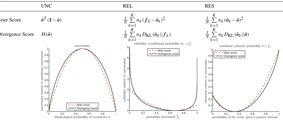
In Weijs et al. (2010), a decomposition of the divergence score was presented that was inspired by a decomposition of the Brier score (Brier, 1950) into uncertainty, reliability and resolution (see Table 1) due to Murphy (1973). This yields the following decomposition:
DS=REL−RES+UNC (4)
DS= 1 N
K
X
k=1
nkDKL(o¯k||fk)− (5)
1 N
K
X
k=1
nkDKL(o¯k|| ¯o)+H (o¯)
whereN is the total number of forecasts andKthe number of unique forecasts issued,nkthe number of forecasts within one category of unique forecasts,o¯k the observed frequency, given forecasts of probabilityfk.
The uncertainty term measures the inherent uncertainty in the climate. The uncertainty reaches a maximum for equiprobable outcomes and is zero if the outcome is always the same. The resolution term measures how much of the climatic uncertainty can be resolved by the forecasts. This is expressed in the average divergence of the conditional distributions of the observations from the marginal distribu-tion of the observadistribu-tions. The reliability measures the aver-age squared distance between the forecast distributions and the corresponding conditional distributions of observations. A perfect reliability of zero (a more accurate term would be unreliability) is attained when for all forecast probabilities, the observed conditional frequency matches that probability. In this case the forecast is said to be perfectly calibrated. 2.2 Interpretations of divergence score and its
decomposition
Table 1. Comparison between the expressions and behaviour of the decompositions of the Brier score and the divergence score for the case
of binary events.
UNC REL RES
Brier Score o¯T(1− ¯o) N1
K
P
k=1
nk(fk− ¯ok)2 N1 K
P
k=1
nk(o¯k− ¯o)2
Divergence Score H (o¯) N1
K
P
k=1
nkDKL(o¯k||fk) N1 K
P
k=1
nkDKL(o¯k|| ¯o)
0 0.2 0.4 0.6 0.8 1 0 0.1 0.2 0.3 0.4 0.5 0.6 0.7 0.8 0.9 1 uncertainty
climatological probability of occurrenceo
u n cer ta in tyr el a ti ve tom a x im u m u n cer ta in ty Brier score Divergence score
0 0.2 0.4 0.6 0.8 1 0 1 2 3 4 5 6
reliability (conditional probabilityok=23)
probablity forecastedfk
re lia b ilit y re la tiv e to u n ce rt a in ty Brier score Divergence score
0 0.2 0.4 0.6 0.8 1 0 0.1 0.2 0.3 0.4 0.5 0.6 0.7 0.8 0.9 1
resolution (climatic probabilityo=1
3)
probability of the event, given a positive forecast
re so lu ti on re la ti ve to u n cer ta in ty Brier score Divergence score
S. V. Weijs et al.: Hydrological forecast evaluation using information theory 15
naive climatological after forecast after recalibration after observation 0 1 re m a in in g u n c e rt a in ty ( B IT S ) U N C R E S D S R E L D S { } t t
( t)
E kl
o D of t{ }
t
( k)
E kl
o D oo t{ ( )}
t t
E kl
o D oo
{ }
t
t
( n)
E kl
o D ou t{ }
t
( )
E kl
[image:5.595.59.546.97.308.2]o D oo
Fig. 1.The remaining uncertainty for different distributions in the forecasting process can be measured by the average Kullback-Leibler divergence from the observations. These uncertainties have some additive relations (DS = UNC−RES + REL).
Fig. 1. The remaining uncertainty for different distributions in the forecasting process can be measured by the average Kullback-Leibler divergence from the observations. These uncertainties have
some additive relations (DS=UNC−RES+REL).
a definition of surprise, a term coined by Tribus (1961). Sur-prise is something we feel when something unexpected hap-pens. The lower the probability we assume something to have, the more surprised we are when observing it. Rain in a desert is surprising, rain in the Netherlands is less sur-prising and rain on the moon is a miracle yielding almost un-bounded surprise. When the surprise of observing outcome x is defined asSx=log(1/P (x)), surprise can be measured in bits like information and uncertainty (Tribus, 1961). Ob-serving something that was a certain fact yields no surprise, heads on a fair coin yield one bit of surprise and observing a 1/1000 year flood in some year yields a surprise of approx-imately 10 bits. The entropy-measure for uncertainty can
now be interpreted as the expected surprise about the truth: H (X)=EX{Sx}, whereEXdenotes the expectation operator with respect to the distribution of random variableX.
In general, uncertainty can now be interpreted as expected surprise about the true outcome. The fact that different ex-pectations can be calculated according to different subjective probability distributions, reflects that uncertainty can be both something objective and subjective. The uncertainty a per-son thinks to have is the entropy of his subjective probability distribution. Kullback-Leibler divergence can be seen as the additional uncertainty one person estimates the other person to have compared to his own:
DKL(P (X)||Q(X))=EP (X){SQ(x)−SP (x)} (6) Because forecast verification is done in hindsight, the obser-vation that is made can be used as a reference point to esti-mate the uncertainty in the forecast. The additional uncer-tainty (expected surprise about the truth), estimated from the viewpoint of the observation is the best available estimate of the remaining uncertainty about the truth of the person hav-ing the forecast. Assumhav-ing perfect observations, the diver-gence score measures remaining uncertainty about the truth and reduces to the logarithmic score (−log[f]j), wherej is the index of the outcome that was observed. We can thus dis-tinguish between this “true” uncertainty, which can only be established in hindsight and the estimated or perceived un-certainty, which is the entropy of the forecast distributionf
of the divergence score relate to the remaining uncertainty at different levels of informedness. Interpreting the figure, res-olution can be seen as the correct information, which can be subtracted from the climatological uncertainty (i.e. the miss-ing information). The reliability term is added to the remain-ing uncertainty and represents the wrong information due to biased probability estimates.
The wrong information can be reduced by calibration. It should be noted that the decomposition is only meaningful when enough data is available to properly calculate all condi-tionals (Weijs et al., 2010). Like calibration of hydrological models to find optimal parameter values, calibration of the forecast distribution needs to re-run the model several times with different settings until the agreement over some histori-cal period is optimal. In the latter case the model is the entire forecasting system consisting of several models, data assim-ilation and statistical post-processing of the forecast distri-bution. Because the meteorological part of the forecasting system is not always accessible for hydrologists and devel-oped continuously, reforecasts of historical meteorology with the most advanced current models are necessary to develop optimally calibrated hydrological forecasts (see also Thielen et al., 2008; Wood and Lettenmaier, 2008).
2.3 Relation between the divergence and Brier scores
The Brier score was introduced by Brier (1950) as a veri-fication score for probabilistic forecasts. It is still the most widely used score for evaluating probabilistic forecasts of bi-nary events.
Given the definitions in the beginning of this section, the Brier score can be defined as:
BSt=2(ft−ot)2=(ft−ot)2: =(ft−ot)T(ft−ot). (7) It must be noted that the Brier score is nowadays almost al-ways defined as half this value (Ahrens and Walser, 2008). To make notation easier, we use the original definition of Brier (see Eq. 7). For a series of forecasts, the Brier score is defined as the average of Eq. (7) over all forecast instances. It can be interpreted as the mean squared error (MSE) in
probabilities.
Murphy (1973) showed that the Brier score for a series of forecasts can be decomposed into uncertainty, resolution and reliability, shown in Table 1. As was found by Weijs et al. (2010), the components of the Brier score are second order approximations of the components of the divergence score (see Table 1). The uncertainty has the same location of maximum and zero points. When scaled with its maxi-mum value, the similarity becomes visible (see left figure in Table 1). The resolution (right figure in Table 1), can reach a maximum equal to the uncertainty term. When scaled with the uncertainty, again a similarity between the shapes of the resolution components is visible. The reliability term, how-ever, exhibits significant differences in the extremes.
While the reliability term of the Brier score is bounded, the analogous term in the divergence score can reach infinity. This happens when an outcome occurs that was given zero probability in the forecast, which are usually extreme events. These events pose a challenge for forecasting: first of all be-cause we have little experience and data for them, making modeling difficult, and secondly because these are events we are not used to cope with and therefore can have severe con-sequences. The divergence score is very sensitive to the cor-rect estimation of the small probabilities for the most unex-pected events, because they contain most information for im-proving the model. When using a forecasting system based on ensembles, reliable probability estimates must be made also outside the range of the most extreme members, for ex-ample by using tools from extreme value statistics. A reli-able probability estimate for an event that is not completely impossible is larger than zero. Unbounded scores will not occur in practice, unless an overconfident forecaster categor-ically rules out something that is possible.
3 Deterministic forecasts cannot be evaluated
Can a forecaster be completely sure about something that in the end does not happen and still get credit for his forecast? This does not appear natural, but it often turns out to hap-pen in practice. For example, a deterministic flow forecast of 200 m3s−1is considered quite good, when 210 m3s−1is observed. Apparently, it is already expected that some error will occur and a forecast that is 10 m3s−1off is considered
to be not that bad. Hydrological models are per definition simplifications of reality. Often, they describe relations be-tween macrostates, like averaged rainfall, mass of water in the groundwater reservoir, and flow through a river cross-section. Similar to problems in statistical thermodynamics, having limited information about what really goes on inside a hydrological system on a microscopical level, our forecasts on a macroscopical level can never be perfect (Weijs, 2009; Grandy Jr., 2008). What can be said about the real world on the basis of a model is therefore inherently erroneous to some extent, or should be stated in terms of probabilities.
positive and removes some of the uncertainty, this is com-pletely annihilated by the reliability term (the wrong infor-mation). The discrepancy between the information (reduc-tion of uncertainty) that the forecasts contain and the infor-mation conveyed by the messages that constitute the fore-casts is so large that the expected surprise about the truth of a person taking the forecast at face value goes to infinity. The fact that deterministic forecasts are still used in society (and unfortunately sometimes even preferred), while they explode uncertainty to infinity, seems to present a paradox. We pro-pose two possible interpretations, one using the information-uncertainty scale and the other using the utility-risk scale, that offer a solution to this paradox.
3.1 Deterministic forecasts are implicitly probabilistic (information interpretation)
Fortunately, in practice, almost no person takes deterministic forecasts at face value. The fact that a user does not take the forecast literally can be seen as recalibration of the forecast (“unconscious statistical post-processing”) by that user. The user bases his internal probability estimates on the forecast, but adjusts the probabilities given by the forecaster based on his own judgment, instead of literally copying the fore-caster’s statements. For a deterministic forecast, this means reallocating some probability to outcomes that the forecast did not speak about. This reallocation improves the reliabil-ity of the internal probabilreliabil-ity estimates of the user on which he bases his actions. We can thus see this as the user eliminat-ing the wrong information from the forecast.1 The user can do the recalibration based on previous experience with the forecasts, common sense and can also add information from his own observations. The user of the forecast can think “if the forecaster says the water level will be 10 cm under the embankment, he implicitly also forecasts a little that over-topping will occur”. Note that the example of Grand Forks in (Krzysztofowicz, 2001) shows that not all users do this. Mathematically this recalibration is equivalent to also attach-ing some probability to overtoppattach-ing. However, it is not the task of a user to guess what the forecaster wanted to say. The forecaster has the task of summarizing different sources of information and expert knowledge into a forecast that vari-ous users can base their decisions on. Consistency requires that the forecaster communicates his judgments to the user (Murphy, 1993). If he deems it possible that 210 m3s−1will flow through the river instead of his best estimate 200 m3s−1, then the forecaster should also communicate a probability for this outcome to the user.
The forecaster may also present the deterministic fore-cast as being an expected value or mean. This suggests
1Note that eliminating wrong information is different from
adding information. If a user takes the forecasts as true, but partial information and is rational (following Bayesian probability logic), no future information can update the zero probability. This is an-other argument against assigning zero probability to anything.
an underlying probabilistic forecast. However, when tak-ing the information-theoretical viewpoint, communicattak-ing an expected value means nothing without additional statements regarding the probability distribution. The principle of maxi-mum entropy (PME) (Jaynes, 1957) states that when making inferences based on incomplete information, the best esti-mate for the probabilities is the distribution that is consis-tent with all information, but maximizes uncertainty. In this way, the uncertainty is reduced exactly by the amount the in-formation permits, but not more. The resulting distribution thus gives an exact representation of the information actually conveyed by the forecast. Maximizing entropy with known mean and variance, gives a Gaussian distribution, maximiz-ing uncertainty about the velocities of gas molecules with known total kinetic energy gives the Boltzmann distribution (Jaynes, 2003; Cover and Thomas, 2006). When PME is applied to expected value forecasts, however, the maximum entropy forecast distribution that is consistent with the infor-mation given by the forecaster is uniform between minus and plus infinity. It is the complete opposite end of the spectrum compared to the previous literal interpretation of the deter-ministic forecast: from claiming total certainty to claiming total uncertainty.
In the case of streamflow forecasts, the user can still get a less nonsensical forecast distribution by combining the information in the forecast with the common sense notion that streamflows in rivers are nonnegative. This extra constraint turns the PME forecast distribution for a known expected value into an exponential distribution (Cover and Thomas, 2006).
This brings back the question who ought to specify these constraints, which constitute information. The fact that the user can reduce the maximum entropy by adding this com-mon sense constraint actually means that the forecaster failed to add this information. Note that the forecaster should be best equipped to give probability estimates and these should be summarized in such a way that no information is lost, but also all uncertainty is represented (cf. consistency).
As was argued in the introduction, predictions only make sense when they are testable, i.e. can be evaluated. One way to evaluate deterministic forecasts with information mea-sures is to convert them to probabilistic forecasts by look-ing at the joint distribution of forecasts and observations. The conditional distributions of observations for each fore-cast value can then be seen as probabilistic forefore-cast distri-butions. It is important to note however, that the probabilis-tic part of such a forecast is derived from data that includes the observations. Such a forecast is thus evaluated against the same data that is used as the basis of its own uncertainty model, which is clearly undesirable.
probabilistic forecast. For example, a deterministic forecast evaluated with root mean squared error implicitly defines a Gaussian forecast probability density function. An important consequence of this insight is that the way to evaluate a de-terministic model actually defines (i.e. forms) the probabilis-tic part of a total model, consisting of a separate determin-istic and probabildetermin-istic part. The objective function (which is a likelihood measure) should therefore be stated a priori, as it forms part of the model that is put to the test against observations.
While estimating the error model from the data may un-der some conditions be acceptable in calibration, for (in-dependent) evaluation of forecasts it is unacceptable, be-cause it uses the data against which it is evaluated. A cor-rect approach would be to explicitly formulate a paramet-ric error model, and find its parameters in the calibration. The combination of the hydrological model and the er-ror model can subsequently be used to make probabilis-tic predictions, which can be evaluated with the divergence score in an independent evaluation period. The error mod-els are not restricted to Gaussian distributions, but can take more flexible forms. Such an approach is taken in Schoups and Vrugt (2010).
As a last consideration, we want to stress that even if an error model is properly formulated and added to the deter-ministic “physical” part, the resulting model still represents a false dichotomy between true behaviour of the system and the error, as was argued by Koutsoyiannis (2010). A more consistent approach would be to explicitly make the proba-bilistic part of the model an integrated part of the physical reality it is supposed to simplify. Such approaches can lie in studying the time-evolution of chaotic systems (Koutsoyian-nis, 2010) or in applying the principle of maximum entropy in combination with macroscopic constraints, as for example suggested by Weijs (2009) and Koutsoyiannis (2005).
Concluding, from the information-theoretical viewpoint, several reasons come to light why deterministic forecasts should in fact be considered to be implicitly probabilistic. The problem with these forecasts is that they leave too much of the probabilistic interpretation to the user. It might be con-sidered ironic that the users who are claimed to not be able to handle probabilistic forecasts and are for that reason pro-vided with deterministic forecasts are the ones who have to rely most on their ability to subconsciously make probability estimates based on the limited information in the determinis-tic forecast.
3.2 Deterministic forecasts can still have value for decisions (utility interpretation)
A second, independent interpretation of deterministic fore-casts that justifies their existence is their usefulness, even to users who do not make subconscious probability esti-mates. Even though a reservoir operator might be infinitely surprised if he has taken a deterministic inflow forecast of
200 m3s−1 at face-value and he finds out the inflow was
210 m3s−1, his loss is not infinite. The operator might spill
some water, but all is not lost.
The difference between surprise and loss is due to the fact that most decision problems are not equal to placing stakes in a series of horse races. Such a horse race is the classical ex-ample where information can be directly related to utility, see Kelly (1956) and Cover and Thomas (2006) for more expla-nation. Kelly showed that when betting on a series of horse races, where the accumulated winnings can be reinvested in the next bet, the stakes the gambler should put on each horse should be proportional to the estimated winning probabili-ties. In a single instance of such a horse race, all money not bet on the winning horse is lost, so the only probability that is important for the results is the one attached to the winning horse. If zero probability (and thus no bets) were put on the winning horse, then the gambler loses all his capital and has no chance of future winnings. In contrast, for decision prob-lems like reservoir operation, an operator blindly believing in an inflow into his reservoir of 200 m3s−1and optimally preparing only for that flow, will automatically also be quite well prepared for 210 m3s−1. Conversely, the preparation on a predicted event, which influences the utility of an outcome, may depend on the entire forecast distribution and not just on the probability of the event that materializes. This makes the loss function non-local (locality is discussed in Sect. 4.1).
Another difference with the horse race is that the total amount of value at stake in hydrological decision making usually does not depend on the previous gains, while the re-sults for the horse race assume that the gambler invests all his previously accumulated capital in the bets. The gambler therefore wants to maximize the product of rates of return over the whole series of bets, while for a reservoir opera-tor, each period offers a new opportunity to gain something from the water, even in case he spilled all his water in the previous month. This is comparable with a gambler whose spouse allows him/her to bet a fixed amount of money each week (Kelly, 1956) and then spends it all in the bar on the same evening without possibility of reinvesting in the next bet. Assuming a utility that increases linearly with the con-sumption of beer bought with the winnings, the best decision is to bet all money on the one horse with the best expected return. Again, one loss is not fatal for the whole series of bets. The gambler just hopes for better luck next week. The evaluation of the value of deterministic forecasts is therefore not as black and white as evaluation of the information they contain.
S. V. Weijs et al.: Information theory for evaluation of hydrological predictions 2553
0 50 100 150 200 250 300 350
0 0.2 0.4 0.6 0.8 1
probability of non−exceedence
Fct A, CRPS = 9.59 Fct B, CRPS = 12.24 observation
0 50 100 150 200 250 300 350
0 0.01 0.02 0.03
streamflow (m3/s)
probability density (s/m
3)
[image:9.595.51.286.65.251.2]Fct A, DS = 4.18 Fct B, DS = 3.92 observation
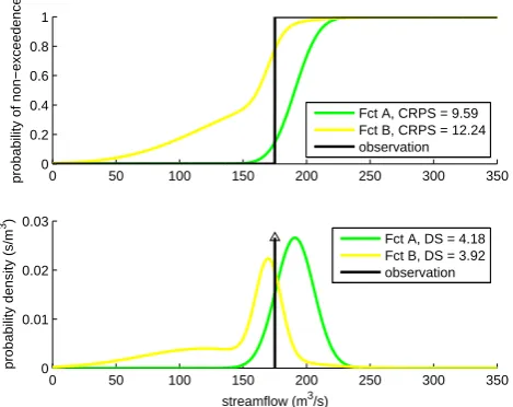
Fig. 2.The RPS and CRPS scores measure the sum of squared differences in CDFs. Therefore they depend on probabilities assigned to events that where not observed. The divergence score only depends on the value of the PDF (the slope of the CDF) at the value of the observation. In the example, forecast A has a better (=lower) CRPS than forecast B, even though it assigned a lower probability to what was observed (resulting in a higher (=worse) DS).
Fig. 2. The RPS and CRPS scores measure the sum of squared
dif-ferences in CDFs. Therefore they depend on probabilities assigned to events that where not observed. The divergence score only de-pends on the value of the PDF (the slope of the CDF) at the value of the observation. In the example, forecast A has a better (=lower) CRPS than forecast B, even though it assigned a lower probability to what was observed (resulting in a higher (=worse) DS).
mean squared error implicitly defines a decision process in which the disutility is a quadratic function of the distance between forecast and observation. In that case, a series of forecasts that has the smallest MSE has most utility or value for the user.
4 Information versus utility as calibration objective
Value-based forecast evaluation (the utility-risk scale) is in-evitably connected to a particular user with a decision prob-lem and therefore cannot be done without explicit consider-ation of the user base of forecasts. Moreover, an obvious question that arises is whether it is desirable to base the eval-uation on the value to a particular user or group of users. In that case, the evaluation becomes an evaluation of the deci-sions of those users rather than of the forecasts themselves or of the hydrological model that produced them. This differ-ence is particularly important if the results of the evaluation are used in a learning or calibration process. In that case, two effects can occur by using value instead of information as a calibration objective:
– The model learns from information that is not there (treated in Sect. 4.1).
– The model fails to learn from all information that is there (treated in Sect. 4.2).
4.1 Locality and philosophy of science
Locality is a property of scores for probabilistic forecasts (Mason, 2008; Benedetti, 2010). A score is said to be lo-cal if the score only depends on the probability assigned to (a small region around) the event that occurred, and does not depend on how the probability is spread out over the values that did not occur. In contrast to this, non-local scores do depend on how that probability is spread out.
Usually non-local scores are required to be sensitive to dis-tance, which means that probability attached to values far from the observed value is punished more heavily than fore-cast probability that was assigned to values close to the ob-servation. This concept of distance only plays a role in fore-casts of continuous and ordinal discrete predictands. For both these types of predictands, an extension of the Brier score ex-ists: the Ranked Probability Score (RPS) and the continuous RPS (CRPS) (see Laio and Tamea, 2007 for description and references). Both these scores are non-local, while the diver-gence score is local.
Figure 2 shows a comparison between (non-local) CRPS and the (local) divergence score. Note that forecast B ob-tains a worse CRPS than forecast A, even though B gives a higher probability to what is actually observed. It can also be imagined how changes in the distribution of the lower tail of forecast B would affect the CRPS, although based on the observation no statements can be made about the merit of that redistribution of probability. Note that any prefer-ence between two forecasts that assign equal probilities to the observed value must be based on prior information (e.g. the fact that a bimodal distribution is counter-intuitive). It is important, however, that this prior information should be in-cluded in the forecast, rather than adding it implicitly during the evaluation process.
For most decision problems, expected utility is a non-local score: a reservoir operator that attached most probability to values far from the true inflow is worse off than one that used a forecast with most probability close to the true value, even if the probability (density) attached to the true value was the same. Therefore, non-local scores are sometimes considered to have more intuitive appeal than local scores. It might seem logical to train a forecasting model to maximize the user-specific utility it yields for the training data, which may be a non-local function.
2554 S. V. Weijs et al.: Information theory for evaluation of hydrological predictions
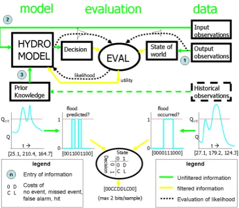
Fig. 3.There are three routes through which information can enter the model in a learning process: the output observations (1), the input observations (2) and prior information (3). When evaluating a model based on value, the decision model that is implicitly defined by the loss function acts as a filter on the information in the observations. The figure shows the case where both the decision and the state of the world are binary, resulting in a feedback of costs to the model of only 2 bits of information per input-output observation pair (the string of characters at the bottom of the figure). The graphs in the middle show how both the predicted and the measured flows are converted to binary sequences due to the way the cost-loss model is formulated.
Fig. 3. There are three routes through which information can
en-ter the model in a learning process: the output observations (1), the input observations (2) and prior information (3). When evaluating a model based on value, the decision model that is implicitly de-fined by the loss function acts as a filter on the information in the observations. The figure shows the case where both the decision and the state of the world are binary, resulting in a feedback of costs to the model of only 2 bits of information per input-output observa-tion pair (the string of characters at the bottom of the figure). The graphs in the middle show how both the predicted and the measured flows are converted to binary sequences due to the way the cost-loss model is formulated.
Changes in the objective function would cause the model to learn something from an evaluation of what is stated about a non-observed event. In an extreme case, two series that forecast the same probabilities for all the events that were observed, can obtain different scores based only on differ-ences in the probabilities assigned to events that were never observed (Benedetti, 2010). A similar argument in the con-text of experimental design was made by Bernardo (1979). If these non-local scores are used as objectives in calibration or inference (see for example Gneiting et al., 2005), things are thus inferred from non-observed outcomes, i.e. information that is not present in the observations.
4.2 Utility as a data filter
The use of utility in calibration can, apart from using non-existing information, also lead to learning only from part of the information that is in the observations. In that sense, the decision problem that specifies the utility acts like a filter on the information. The information-theoretical data processing inequality tells us that this filter can only decrease informa-tion (see Cover and Thomas, 2006). This filter can affect two of the three information flows to the model, depicted in Fig. 3: the flow from the output (1) and from the input (2) observations.
The first flow of information (from the observations of streamflow) is filtered by the “state of world” block in Fig. 3. By evaluating based on utility, the information in the stream-flow observations only reaches the model through its effect on how the state of the world affects the utility of decisions based on the forecast. Figure 3 depicts a hypothetical binary evacuation decision that is coupled to a conceptual rainfall-runoff model for flood forecasting. In this simplified decision problem, the utility is only influenced by a binary decision (evacuate or not) and a binary outcome (the place floods or not). There are thus no gradations in severity of the floods that affect the damage. The calibration towards maximum utility for this decision problem will train the hydrological model to optimally distinguish flood-evacuation events. This implies that in the training, all that the hydrological model sees from the continuous observed discharges is a binary sig-nal: flood or no flood. This constitutes at most one bit of information per observation (in the unlikely case that 50% of the observations is above the flood threshold, i.e. the cli-matic uncertainty is 1 bit), while the original signal (the ob-served flows i.e. real numbers) contained far more informa-tion (see Fig. 3).
The second flow of information to the model, the input ob-servations, is affected by the information filter in the “deci-sion” block. For example, if a binary decision problem (e.g. to be or not to be in the flood zone tomorrow) is considered, the information from input observations travels through the model and subsequently through the decision model. While the model still gives a real number as output, the “decision” block maps that model output to a binary signal (to be or not to be). The binary signal is all that enters the evaluation and can be learned from the input observations. When a model is evaluated based on a cost-loss model of a two action- two state of the world decision problem, the maximum amount of information that can be learned from each input-output observation pair is thus 2 bits. In Fig. 3, this information is contained in the string “00CCDDLC00”, which represents the sequence of utilities over all time steps.
evacuation decisions could benefit from more parsimonious data-driven models (e.g. linear regression models or neural networks). These models can make a mapping directly from predictors (e.g. precipitation, snowpack, soil moisture, past discharge) to decisions, but this complicates the use of prior information.
The third information flow in Fig. 3 consists of this prior information on the workings of the hydrological system, which can be valuable for improving forecasts. The infor-mation can enter in the form of prior parameter estimates or constraints that are captured in the model structure. Exam-ples are constraints on mass balance and energy limits for evaporation. These constraints describe the patterns in data or “physical laws” that ultimately come from observations. Both adding too much (unwarranted assumptions) and too little (e.g. too wide prior parameter distributions) informa-tion through this route deteriorates the forecasts, especially when little data is available.
The framework presented in this section shows some sim-ilarity with the ideas presented in (Gupta et al., 2009, 1998, 2008). In those papers it is also argued that information can be lost in the evaluation. However, the important difference of this framework compared to those ideas is that we argue that information is lost by using measures other than infor-mation (in other words, measures that do not reflect likeli-hood), while Gupta et al. (2008) argue that information is lost because of the low dimensionality of the evaluation measure. In our information-theoretical viewpoint, we can in princi-ple learn all we need from the observations through a single measure (a real number can contain infinitely many bits of information). What is learned depends only on the data and the prior information. The challenge is to give a reliable rep-resentation of prior information which will result in the right likelihood function. In principle, this is equivalent to endors-ing the likelihood principle, which states that all information that the data contains about a model is in the likelihood func-tion, as argued by Robert (2007) p. 14, Jaynes (2003) p. 250 and Berger and Wolpert (1988).
[image:11.595.309.548.133.175.2]The divergence score (which can be seen as log-likelihood) corresponds to a logarithmic scoring rule (see Jose et al., 2008), which is the only scoring rule that is both local and proper (proofs can be found in Bernardo, 1979 and Benedetti, 2010), where propriety is the requirement that the scoring rule can only be optimized when the forecaster does not lie. Scoring rules that are not proper can be hedged, meaning that the expected score is maximized by forecasting probabilities that are not consistent with the best estimates of the forecaster (see Gneiting and Raftery (2007) for an elab-orate discussion on proper scoring rules). A utility function that includes the importance of the outcomes can be hedged by attaching more forecast probability to important events. A model that is trained on such a measure is thus encouraged to “lie”. All utility functions that are not affine functions of information violate either locality or propriety, which makes them doubtful objectives for calibration.
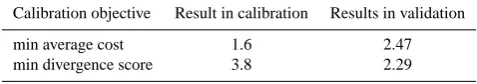
Table 2. The resulting average disutility per year, composed of
costs for action and losses for unpredicted events, is minimized by explicitly calibrating on it, but performance in the validation period is better for the probabilistic model trained to minimize remaining uncertainty.
Calibration objective Result in calibration Results in validation
min average cost 1.6 2.47
min divergence score 3.8 2.29
4.3 Practical example
As an illustration of the information-filter effect described in Sect. 4.2, a hydrological model was calibrated both based on information and on a utility function relating to the bi-nary decision scenario similar to that depicted in Fig. 3. A simple lumped conceptual rainfall-runoff model was used (Schoups et al., 2010) to simulate daily streamflow given daily forcing records of rainfall and evaporation from the French Broad River basin at Asheville, North Carolina. The model was calibrated using 1 year of streamflow observa-tions (1961), and validated using 9 years of streamflow ob-servations (1970–1978).
The calibration on the information-uncertainty scale used minimization of the divergence score (i.e. remaining uncer-tainty) as an objective. In the continuous case this cor-responds to maximizing the log-likelihood. This means that the model needs to provide explicit probabilistic fore-casts. The probabilistic part of the model used a flexible stochastic description, allowing for heteroscedasticity, au-tocorrelation and non-Gaussian distributions. The calibra-tion relied on the general likelihood funccalibra-tion presented in Schoups and Vrugt (2010).
The calibration on the utility-risk scale employed a cost-loss utility function relating to the binary decision problem (Murphy, 1977). The flood threshold is defined at a value of 10 mm d−1(streamflow divided by catchment area). Here,
a cost C is associated with a precautionary action, which is taken if exceedence of the flood threshold is forecast. When a peak flow event occurs but was not predicted, a loss L occurs. For illustration purposes, values for C and L were chosen to be equal to 0.2 and 1.0, respectively.
2556 S. V. Weijs et al.: Information theory for evaluation of hydrological predictions these parameters gave an advantage in fitting the floods in the
calibration year. In contrast, the probabilistic model is en-couraged to attach high likelihood to each observation, learn-ing from all data in the calibration. In this case, this gave an advantage in predicting the exceedance probability for the flood threshold for the unseen validation data.
We must note, however, that results might be different un-der less ideal conditions. For example, when the model struc-ture is capable of representing high flows, but is inadequate for low flow situations because e.g. evaporation is not cor-rectly represented, then the utility-based calibration might do better also in validation. We can explain this by seeing the utility function as an implicit way to add prior information. If we know a priori that the model structure misses relevant processes for low flow, then it could be reasonable to ignore the low-flow data in calibration. The analogous way to rep-resent this in an explicit uncertainty model is to give an extra spread to the probabilistic predictions at low flows, making the model less sensitive to them. More elaborate case stud-ies are needed to further investigate which practical factors might lead to different results and how they can be accounted for in the information-theoretical framework. Furthermore, applying this view on results in past literature, especially those relating to “informal” likelihood methods, might give new insights about prior information that is implicitly added.
5 Conclusions
The difficulties and debate about the evaluation of forecasts can be significantly clarified using an information-theoretical viewpoint. It shows why forecasts should be probabilis-tic and why measuring their quality on the information-uncertainty scale is important. When information is seen as a measurable quantity, like energy, a sort of “informa-tion intui“informa-tion” develops, similar to the “energy intui“informa-tion” that is used to detect logical flaws in claims for perpetuum mo-biles. For the interesting connection between energy and in-formation, see e.g. (Toyabe et al., 2010). Science is required to make testable predictions. Forecasts should therefore be stated in terms that make it clear how to evaluate them. De-terministic and interval forecasts fail this criterion, because additional assumptions on utility and probability have to be made during evaluation of the forecast. Probabilistic fore-casts can be evaluated using information theory. The de-composition of the divergence score that was presented in Weijs et al. (2010) can provide additional insight in the inter-action between uncertainty, correct information and wrong information.
Starting from the observation that deterministic forecasts are still commonly used and evaluated, but are worthless from an information-theoretical viewpoint, we draw the con-clusion that these forecasts are either implicitly probabilistic or should be viewed in connection to a decision problem. In both interpretations, the evaluation depends on external
in-26000 2640 2680 2720 2760 2800
4 8 12 16
Time (days)
Streamflow (mm/d)
flood threshold
20 and 80% quantiles probabilistic model utility based calibration
[image:12.595.309.545.63.182.2]observations
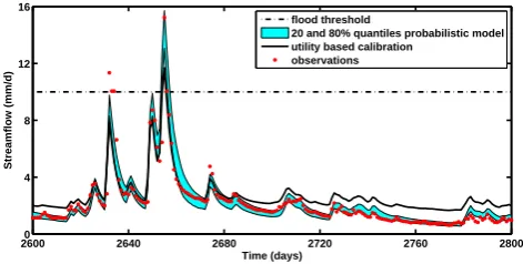
Fig. 4.The results from both models, compared with observations. For the probabilistic model, the 20% and 80% quantiles are shown. With the cost-loss ratio of 0.2 used in this example, the upper quantile determines the decision.
Fig. 4. The results from both models, compared with observations.
For the probabilistic model, the 20% and 80% quantiles are shown. With the cost-loss ratio of 0.2 used in this example, the upper quan-tile determines the decision.
formation that is not provided in the forecast. Deterministic forecasts leave too much interpretation to the user, if seen as implicit probabilistic forecasts, or make too many assump-tions on the user if they are evaluated using another utility measure.
On the one hand, forecasting can be seen as a com-munication problem in which uncertainty about the out-come of a random event is reduced by delivering an informative message to a user. On the other hand, fore-casting can be seen as an addition of value to a deci-sion problem. Any measure that is not information only becomes meaningful when it is interpreted in terms of util-ities. When addressing forecast value, it is important to see that in fact we are evaluating decisions based on forecasts and not the correspondence between the observations and the forecasts themselves.
This is especially important in calibration, where a model has to learn from observations. When calibration objectives are used that are not information-measures, the model ei-ther learns from information that is not ei-there or uses only part of the information in the observations, or both. Be-cause the amount of available information is related to opti-mal model complexity, hydrological models trained for user specific utilities are more prone to overfitting, which might lead to worse results in an independent validation test. 5.1 Avenues for future research
experimentally is to estimate models from data under vary-ing conditions, usvary-ing both artificial data and real world data. Various calibration objectives can then be compared to see how practical results support the theory.
Another important and interesting point to study is the role of model complexity. This paper has only looked at the per-formance of models in predicting the observations. When an overly complex model is trained to do this optimally, it will attain very good results in calibration but do not so well in validation. This is a result of the model having such a high complexity that it starts to extract information from incidental rather than from general patterns in the relation between the variables that is to be modeled. Information-theoretical measures are well suited to be combined with model complexity measures. An interesting point to note in this respect is that the Akaike information criterion (Akaike, 1974) consists of a term for model complexity plus a term for model performance that is actually equal to the diver-gence score. Beyond this information criterion there are even deeper (but less practical) theories from algorithmic informa-tion theory, independently discovered by Solomonoff (1964); Chaitin (1966); Kolmogorov (1968). In principle, these the-ories contain the building blocks for a more complete frame-work for model inference, considering the amount of infor-mation in the calibration data, the optimal complexity of a model and maximum extraction of information from the data. An important open question is how to consistently add prior information about the model structure without being over-confident about the validity of this information. Further-more, theoretical work on the concept of sufficiency (Ehren-dorfer and Murphy, 1988) within the presented information-theoretical framework might prove interesting.
On the practical side, further research could test the ap-plicability of the ideas presented here in the context of en-semble flood forecasting. An interesting topic is for ex-ample how to assign reliable probabilities in the tails of the forecast distributions. This is neccesary to increase the acceptance of the logarithmic scoring rule, given its high sensitivity for overconfident wrong predictions. Code for the divergence score decomposition is freely available on divergence.wrm.tudelft.nl.
Acknowledgements. The authors thank Ronald van Nooijen and Luciano Raso for fruitful discussions about the manuscript. We also thank the anonymous reviewer and Federico Lombardo for their constructive and thought-provoking comments.
Edited by: D. Koutsoyiannis
References
Ahrens, B. and Walser, A.: Information-based skill scores for prob-abilistic forecasts, Mon. Weather Rev., 136, 352–363, 2008. Akaike, H.: A new look at the statistical model identification, IEEE
transactions on automatic control, 19, 716–723, 1974.
Bartholmes, J. C., Thielen, J., Ramos, M. H., and Gentilini, S.: The european flood alert system EFAS – Part 2: Statistical skill as-sessment of probabilistic and deterministic operational forecasts, Hydrol. Earth Syst. Sci., 13, 141–153, doi:10.5194/hess-13-141-2009, 2009.
Benedetti, R.: Scoring Rules for Forecast Verification, Mon.
Weather Rev., 138, 203–211, 2010.
Berger, J. and Wolpert, R.: The likelihood principle, Institute of Mathematical Statistics, Hayward, CA, 2nd edn., 1988. Bernardo, J.: Expected information as expected utility, The Annals
of Statistics, 7, 686–690, 1979.
Brier, G. W.: Verification of forecasts expressed in terms of proba-bility, Mon. Weather Rev., 78, 1–3, 1950.
Br¨ocker, J. and Smith, L.: Scoring probabilistic forecasts: The im-portance of being proper, Weather Forecast., 22, 382–388, 2007. Chaitin, G.: On the length of programs for computing finite binary
sequences, Journal of the ACM (JACM), 13, 547–569, 1966. Cover, T. and Thomas, J.: Elements of information theory,
Wiley-Interscience, New York, 2006.
Ehrendorfer, M. and Murphy, A.: Comparative evaluation of
weather forecasting systems: Sufficiency, quality, and accuracy, Mon. Weather Rev., 116, 1757–1770, 1988.
Gneiting, T. and Raftery, A.: Strictly proper scoring rules, predic-tion, and estimapredic-tion, J. Am. Stat. Assoc., 102, 359–378, 2007. Gneiting, T., Raftery, A., Westveld, A., and Goldman, T.:
Cal-ibrated probabilistic forecasting using ensemble model output statistics and minimum CRPS estimation, Mon. Weather Rev., 133, 1098–1118, 2005.
Grandy Jr., W.: Entropy and the Time Evolution of Macroscopic Systems, Oxford University Press, New York, 2008.
Gupta, H., Kling, H., Yilmaz, K., and Martinez, G.: Decomposition of the mean squared error and NSE performance criteria: Impli-cations for improving hydrological modelling, J. Hydrol., 377, 80–91, 2009.
Gupta, H. V., Sorooshian, S., and Yapo, P. O.: Toward improved calibration of hydrologic models: Multiple and noncommensu-rable measures of information, Water Resour. Res., 34, 751–763, 1998.
Gupta, H. V., Wagener, T., and Liu, Y.: Reconciling theory with observations: elements of a diagnostic approach to model evalu-ation, Hydrol. Process., 22, 3802–3813, 2008.
Jaynes, E.: Probability theory: the logic of science, Cambridge Uni-versity Press, Cambridge, UK, 2003.
Jaynes, E. T.: Information Theory and Statistical Mechanics, Phys-ical Review, 106, 620–630, 1957.
Jolliffe, I. T. and Stephenson, D. B.: Forecast verification: a prac-titioner’s guide in atmospheric science, Wiley, Chichester, UK, 2003.
Jose, V., Nau, R., and Winkler, R.: Scoring rules, generalized entropy, and utility maximization, Oper. Res., 56, 1146–1157, 2008.
Kelly, J.: A new interpretation of information rate, Information The-ory, IEEE Transactions on, 2, 185–189, 1956.
Kolmogorov, A.: Three approaches to the quantitative definition of information, Int. J. Comput. Math., 2, 157–168, 1968.
Hydrol. Earth Syst. Sci., 14, 585–601, doi:10.5194/hess-14-585-2010, 2010.
Krzysztofowicz, R.: The case for probabilistic forecasting in hy-drology, J. Hydrol., 249, 2–9, 2001.
Laio, F. and Tamea, S.: Verification tools for probabilistic forecasts of continuous hydrological variables, Hydrol. Earth Syst. Sci., 11, 1267–1277, doi:10.5194/hess-11-1267-2007, 2007. Mason, S.: Understanding forecast verification statistics, Meteorol.
Appl., 15, 31–40, 2008.
Montanari, A. and Brath, A.: A stochastic approach for assess-ing the uncertainty of rainfall-runoff simulations, Water Resour. Res., 40, W01106, doi:10.1029/2003WR002540, 2004. Montanari, A., Shoemaker, C., and van de Giesen, N.: Introduction
to special section on Uncertainty Assessment in Surface and Sub-surface Hydrology: an overview of issues and challenges, Water Resour. Res., 45, W00B00, doi:10.1029/2009WR008471, 2009. Murphy, A.: The value of climatological, categorical and proba-bilistic forecasts in the cost-loss ratio situation, Mon. Weather Rev., 105, 803–816, 1977.
Murphy, A. H.: A new vector partition of the probability score, J. Appl. Meteorol., 12, 595–600, 1973.
Murphy, A. H.: What is a good forecast?: An essay on the nature of goodness in weather forecasting, Weather Forecast., 8, 281–293, 1993.
Oreskes, N., Shrader-Frechette, K., and Belitz, K.: Verification, val-idation, and confirmation of numerical models in the earth sci-ences, Science, 263, 641–646, 1994.
Peterson, M. B.: An introduction to decision theory, Cambridge University Press, Cambridge, UK, 2009.
Ramos, M., Mathevet, T., Thielen, J., and Pappenberger, F.: Com-municating uncertainty in hydro-meteorological forecasts: mis-sion impossible?, Meteorol. Appl., 17, 223–235, 2010.
Robert, C.: The Bayesian choice: from decision-theoretic foun-dations to computational implementation, Springer Verlag, New York, 2007.
Schoups, G. and Vrugt, J.: A formal likelihood function for param-eter and predictive inference of hydrologic models with corre-lated, heteroscedastic, and non-Gaussian errors, Water Resour. Res, 46, W10531, doi:10.1029/2009WR008933, 2010.
Schoups, G., van de Giesen, N. C., and Savenije, H. H. G.: Model complexity control for hydrologic prediction, Water Resour. Res, 44, W00B03, doi:10.1029/2008WR006836, 2008.
Schoups, G., Vrugt, J., Fenicia, F., and van de Giesen, N.: Cor-ruption of accuracy and efficiency of Markov chain Monte Carlo simulation by inaccurate numerical implementation of conceptual hydrologic models, Water Resour. Res, 46, W10530, doi:10.1029/2009WR008933, 2010.
Shannon, C. E.: A mathematical theory of communication, Bell System Technical J., 27, 379–423, 1948.
Solomonoff, R.: A formal theory of inductive inference. Part I, In-form. Control, 7, 1–22, 1964.
Thielen, J., Schaake, J., Hartman, R., and Buizza, R.: Aims, chal-lenges and progress of the Hydrological Ensemble Prediction Ex-periment (HEPEX) following the third HEPEX workshop held in Stresa 27 to 29 June 2007, Atmos. Sci. Lett., 9, 29–35, 2008. Thirel, G., Martin, E., Mahfouf, J.-F., Massart, S., Ricci, S.,
Regim-beau, F., and Habets, F.: A past discharge assimilation system for ensemble streamflow forecasts over France – Part 2: Impact on the ensemble streamflow forecasts, Hydrol. Earth Syst. Sci., 14, 1639–1653, doi:10.5194/hess-14-1639-2010, 2010.
Tribus, M.: Thermostatics and thermodynamics, D. Van Nostrand Company, Inc, 1961.
Toyabe, S., Sagawa, T., Ueda, M., Muneyuki, E., and Sano, M.: Ex-perimental demonstration of information-to-energy conversion and validation of the generalized Jarzynski equality, Nat. Phys., 6, 988–992, doi:10.1038/nphys1821, 2010.
Von Neumann, J. and Morgenstern, O.: Theory of games and eco-nomic behavior, Princeton University Press, third edn., 1953. Weijs, S.: Interactive comment on “HESS Opinions ‘A random
walk on water’ ” by: Koutsoyiannis, D., Hydrol. Earth Syst. Sci. Discuss., 6, C2733–C2745, 2009.
Weijs, S., Van Nooijen, R., and Van de Giesen, N.: Kullback– Leibler divergence as a forecast skill score with classic reliability-resolution-uncertainty decomposition, Mon. Weather Rev., 138, 3387–3399, 2010.
Wilks, D. S.: Statistical methods in the atmospheric sciences, Aca-demic Press, San Diego, CA, 2nd edn., 2006.