Geophysical methods to support correct water sampling locations for salt dilution gauging

www.hydrol-earth-syst-sci.net/18/3195/2014/ doi:10.5194/hess-18-3195-2014

© Author(s) 2014. CC Attribution 3.0 License.

Geophysical methods to support correct water sampling locations

for salt dilution gauging

C. Comina1, M. Lasagna1, D. A. De Luca1, and L. Sambuelli2

1_{Dept. of Earth Science (DST), Università degli Studi di Torino, via Valperga Caluso, 35, 10125 Turin, Italy}

2_{Dept. of Environment, Land and Infrastructure Engineering (DIATI), Politecnico di Torino, corso Duca degli Abruzzi, 24,} 10129 Turin, Italy

Correspondence to: C. Comina ([email protected])

Received: 8 May 2014 – Published in Hydrol. Earth Syst. Sci. Discuss.: 19 May 2014 Revised: – – Accepted: 24 July 2014 – Published: 26 August 2014

Abstract. To improve water management design, particu-larly in irrigation areas, it is important to evaluate the base-line state of the water resources, including canal discharge. Salt dilution gauging is a traditional and well-documented technique in this respect. The complete mixing of salt used for dilution gauging is required; this condition is difficult to test or verify and, if not fulfilled, is the largest source of un-certainty in the discharge calculation. In this paper, a geo-physical technique (FERT, fast electrical resistivity tomog-raphy) is proposed for imaging the distribution of the salt plume used for dilution gauging at every point along a sam-pling cross section. With this imaging, complete mixing can be verified. If the mixing is not complete, the image created by FERT can also provide a possible guidance for selecting water-sampling locations in the sampling cross section. A water multi-sampling system prototype aimed to potentially take into account concentration variability is also proposed and tested.

The results reported in the paper show that FERT provides a three-dimensional image of the dissolved salt plume and that this can potentially help in the selection of water sam-pling points.

1 Introduction

Improved management of water resources is becoming more important as several areas of the world suffer from water shortages. Therefore, correct evaluation and preservation of water resources is essential. An important starting point for

improving management design is to evaluate the baseline state of the resources, including the amount of discharge from watercourses and irrigation canals.

The most common approach for measuring discharge is the velocity–area method, which involves measuring water depth and velocity at points across a stream section with a current meter. An alternative method of stream gauging in-volves the injection of a chemical tracer and the evaluation of its dilution following its complete mixing into the stream (Rantz, 1982). This last method is often referred to as di-lution gauging: for example the measure of electrical con-ductivity (EC) as a function of time in a measuring section is performed and related to ion concentration; this last measure-ment is integrated over time to obtain the discharge value.

Dilution gauging is frequently used in open channels to investigate superficial flows, especially in mountainous streams where the irregular, boulder-laden cross sections and the strong turbulence decrease the accuracy with which depth and velocity can be measured (Moore, 2004; Radulovic et al., 2008). Different types of tracers have been used for dilution gauging; NaCl (in ionic form) is the most frequently used one (Drost, 1989; Zellweger, 1994; Kumar and Nachiappan, 2000; Tazioli, 2011).

3196 C. Comina et al.: Geophysical methods to support correct water sampling locations for salt dilution gauging

measuring equipment is very easy to move. The only disad-vantage of this last methodology is the amount of NaCl that needs to be added that is primarily linked to the background EC level; different discussions can be found in the literature in this respect (Gees, 1990; Kite, 1993; Hudson and Fraser, 2002; Moore, 2005).

An important issue of dilution gauging is that the method requires a complete vertical and lateral mixing of the tracer at the sampling site, without tracer losses or gains between the injection site and the measurement site. Vertical mixing typ-ically occurs more rapidly than lateral mixing (Rantz, 1982). The dynamics of mixing will vary based on the hydraulic characteristics of the given reach. Frequently, long reaches are needed to ensure a complete lateral mixing of the tracer. An optimum mixing length is generally the one that allows for adequate mixing but does not require an excessively long sampling duration. When the slug injection method is used, complete mixing is considered to have occurred when the concentration is uniform at every point of the cross section at the sampling location. If the adequate mixing is not cer-tain at a given sampling location, the tracer must be sam-pled for its entire transit time at several locations throughout the sampling cross section of the channel. Rantz (1982) has found that at least three lateral sampling points should be used regardless of stream characteristics. Several empirical equations that take into account the different canal features (gross estimated discharge, width, etc.) and the type of tracer injected can be found in the literature to determine the mixing length (e.g., Moore, 2005; Jaramillo, 2007). These equations commonly provide inaccurate estimates as they often under-estimate the mixing length. Apart from these specifications, no particular precautions are proposed in the literature for directly verifying the complete lateral and vertical mixing of the tracer.

Indirect geophysical measurements, such as electrical re-sistivity tomography (ERT), can potentially be applied to evaluate mixing. ERT usage has been developed in recent decades as a monitoring tool (Xie et al., 1995; Tapp and Wilson, 1997) and can be profitably used to image compo-nent concentration distributions and detect dynamic changes in a multi-phase processes. Moreover, quantitative evalua-tions about the properties of the imaged water can be ac-complished using one of the various relationships relating the electrical resistivity to the physical and chemical properties of the water mixture. Most of the applications presented in the literature (Fangary et al., 1998; Lucas et al., 1999; Wang and Cilliers, 1999; Yang and Liu, 2000; Warsito and Fan, 2001) address cylindrical flows (in pipes, cyclones, tanks), and the electrodes are placed on one or more circumferences orthogonal to the cylinder axis. This geometrical configura-tion assures an optimum condiconfigura-tioning of the inverse tomo-graphic problem, but its applicability to real case studies on natural rivers or channels is limited. A number of previous studies have focused on situations where the imaged body cannot be entirely surrounded by electrodes, as in the case of

creeks, rivers and canals. This has been performed in slow water flows (Sambuelli et al., 2002) to assess the possibility of recognizing the presence of granular materials and in fast water flows in the laboratory (Sambuelli and Comina, 2010) to image solid and pollutants flowing through a canal cross section. In this last application the fast electrical resistivity tomography (FERT), proposed in this work, has been already tested under controlled conditions. FERT has the advantage of allowing for very fast monitoring of the flow due to the high speed of acquisition of the tomographic images. This capability extends the field of applicability of common ERT methods.

The objective of this study is to evaluate the potential of FERT to image the cross-sectional distribution of an NaCl (in ionic form) plume, used for dilution gauging, in a real case study. Because the knowledge of tracer distribution through-out the measuring cross section is crucial to correctly posi-tion the sampling points, FERT can be potentially used as a preliminary control. Providing an image of the plume would help in selecting appropriate sampling points and establish-ing a more accurate section for dilution gaugestablish-ing. FERT im-ages are also compared with direct local measures of the same NaCl (in ionic form) plume. These are performed by means of a water multi-sampling system prototype developed for simultaneous sampling at different points along the cross section. A comparison of the results is discussed with the aim of evaluating the potential of FERT as a guide for the correct location of water sampling points.

2 Methods

After a brief introduction to the test site, the conceptual basis and field procedures for slug injection using dilution gauging and geophysical controls are hereafter presented. In particular, the water multi-sampling system prototype, pro-posed for the optimization of tracer detection, is described together with the field procedures necessary for the execu-tion of FERT.

2.1 The study area: the Osasco Canal

Figure 1. Geographical location of the test canal (inlet) and a more detailed view in the proximity of the test site.

length estimated from empirical relationships (Moore, 2005; Jaramillo, 2007) is approximately 50 m. To ensure an ad-equate testing length, a canal reach of 100 m was chosen (Fig. 1).

Pictures of both the sampling and the injection points are shown in Fig. 2. In the studied reach the bottom of the chan-nel is cobbled (gravel and cobbles), except for a small portion immediately upstream of the chosen injection point, where a small cemented weir is located (Fig. 2). The measuring sec-tion is located under a small road bridge, and a canal curve is located immediately downstream of this section (Fig. 2).

The most appropriate reach was chosen considering the following: (1) the reach has no dead water between the in-jection and sampling points; (2) the sampling site is free of air bubbles caused by excessive turbulence that interfere with EC measurements; (3) the injection point appears to be turbu-lent enough to ensure the tracer mixing; (4) the background EC level of the river is stable during the measuring time; (5) the reach length is consistent with the estimated mixing length.

2.2 Slug injection method

In this study NaCl (in ionic form) was used as a tracer: a mass of 9 kg was dissolved in a barrel in approximately 30 L of water and was instantaneously injected into the canal at the injection point (Fig. 2). Fluorescein was also added to the salt–water mixture to have a qualitative visualization of its passage in the measuring section. The basic principle is that the ionic NaCl concentration in the slug increases the natu-ral water concentration; this increases the measured electrical conductivity (EC), which can be used as an index of the salt concentration. Over a wide range of concentrations, the EC is indeed linearly related to salt concentration (Radulovic et al., 2008; Moore, 2005; Gees, 1990; Rantz, 1982) so that the EC response can be transformed in ionic concentration of NaCl.

Figure 2. Tested canal reach: (a) injection point at the end of a

cemented weir and (b) measuring section, under a small road bridge and before a canal curve.

The equation for computing stream discharge, which is based on the principle of the conservation of mass, is (Rantz, 1982)

Q= V0·C0

∞ R

0

(Ct−Cb)dt

, (1)

3198 C. Comina et al.: Geophysical methods to support correct water sampling locations for salt dilution gauging

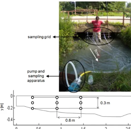
Figure 3. Multi-sampling system with details of the sampling grid

(black circles are water spilling points) and of the pumping appara-tus; the bottom section is seen from upstream.

sampling site andCb[−] is the background concentration of the canal.

The term

∞ R

0

(Ct−Cb)dtrepresents the total area under the concentration–time curve. To obtain this curve the passage of the entire tracer plume was monitored by measuring the EC of the water at the sampling section at a sampling interval of 5 s. Measurements were continuously recorded for approxi-mately 5 min during the passage of the salt plume. The values of the EC curve were then transformed into concentrations through the use of a laboratory-estimated calibration curve. This calibration was constructed by measuring the variation of EC in a sample of the canal water to the addition of dif-ferent amounts of NaCl. The concentration with respect to the natural water conductivity, which is used as reference, is therefore obtained. A highly coherent calibration curve with anRsquared value almost near unity has been obtained:

C =5.3×10−4·σ −9.6×10−2, (2)

whereC is incremental ionic concentration of NaCl [g L−1] andσis conductivity [µS cm−1].

2.3 Sampling optimization

To obtain an EC value that is more representative of the entire sampling cross section, a water multi-sampling system pro-totype was devised. This system was created with a frame-work of steel rods to which nine tubes with a small diame-ter are connected. The tubes are attached to a single wadiame-ter pump which spills the water simultaneously from the nine

Figure 4. Electrodes disposition for cross-flow FERT: images of

the electrodes and the anchoring system (top panel) and of the mesh used for the inversion (bottom panel); the bottom section is seen from upstream.

measuring points – mixing all nine samples and producing an average value at each sample interval. This apparatus al-lows for a more extended sampling of the whole canal sec-tion and reduces, through averaging, the uncertainty due to an incomplete tracer mixing. However, the geometry of the measured section (different water depths along it) and the limited manoeuvrability of the whole system allowed for the sampling of only a portion of the canal section. A scheme of the adopted multi-sampling system and of its location is reported in Fig. 3.

2.4 Cross-flow FERT

Cross-flow FERT has been implemented by means of an ar-ray of 16 underwater electrodes (14 on the canal bottom and 2 on the sides). The electric cable has been anchored on the canal bottom by means of appropriate weights, and the posi-tion of each electrode together with the shape of the secposi-tion has been measured. The electrode positioning scheme for the test site and a picture of the array is shown in Fig. 4.

C. Comina et al.: Geophysical methods to support correct water sampling locations for salt dilution gauging 3199

the collected data, we used a software (NES Electric Arbi-trary 2-D Closed Geometry by Andrea Borsic) based on a damped least-squares inversion algorithm.

A time-lapse analysis calculating the relative difference in electric resistivity (ER) of the acquired images during the plume transit with respect to a reference image was then per-formed. The reference image was achieved from the mean of three FERT measurements carried out before the slug injec-tion (ER of 58m coherently corresponding to the inverse of the EC of 170 µS cm−1 directly measured in the canal). With this representation, the passage of the salt plume is ex-pected to show an overall reduction in resistivity (increased concentration of the salt plume) throughout the images. The same laboratory calibration curve used for dilution gauging was subsequently used to convert the resistivity images in salt concentration images.

3 Results

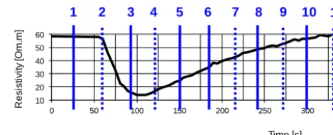
The measured breakthrough curve from the direct sampling with the adopted multi-sampling system is reported in Fig. 5; for convenience of comparison with the results of cross-flow FERT, the data have been converted in ER. The discharge, evaluated with Eq. (1), resulted in 0.46 m3s−1. The main peak evidenced from this curve was approximately 14 m corresponding to an EC of approximately 700 µS cm−1and to a peak concentration of 0.27 g L−1. In Fig. 5, the times when the FERT images were acquired are also reported.

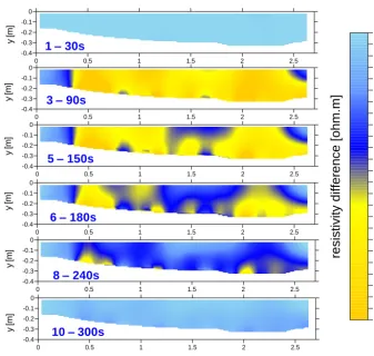
The results of some FERT images during the passage of the salt plume are presented in Fig. 6; some of the images, with very similar ER distributions, have been suppressed (dashed lines in Fig. 5) to simplify visualization. In these im-ages the ER differences with respect to the condition without artificial tracer are reported. The images show clear evidence of the passage of the salt plume, correctly identified with a strong resistivity reduction. This reduction is quite homoge-neous at early times, corresponding to the higher salt concen-tration in the plume, but appears more concentrated in some zones of the canal in the tail of the plume. The left side of the reconstructed resistivity image (which is upstream of the canal curve) appears not to be affected by the passage of the plume. This has also been observed on site by visual inspec-tion of the passing colored plume. The reducinspec-tion in resistivity has an average value of approximately−25m with respect to the clear water, even if localized, more marked reduc-tions (approximately −30–35m) are present in the map. As expected, mainly due to the different sampling time (see also discussion below), the average reduction is a little lower than what was obtained from the direct sampled curve which instead reports a peak reduction of approximately −40m with respect to the canal resistivity without artificial tracer (from 58m to approximately 14m; Fig. 5).

The resistivity images acquired have been then trans-formed to extract quantitative information about the salt

24 and the anchoring system (top) and of the mesh used for the inversion (bottom), the 508

below section is seen from up-stream. 509

510

10 20 30 40 50 60

0 50 100 150 200 250 300 350

1

R

e

si

st

ivi

ty

[O

m

.m

]

Time [s]

2 3 4 5 6 7 8 9 10 11

511

Figure 5. Time-resistivity curve determined with the multisampling apparatus 512

and indication of the number and time of execution of the cross-flow FERT images 513

presented in Figure 7 and 8 (full lines).

514 Figure 5. Time–resistivity curve determined with the

multi-sampling apparatus and indication of the number and time of ex-ecution of the cross-flow FERT images presented in Figs. 7 and 8 (full lines).

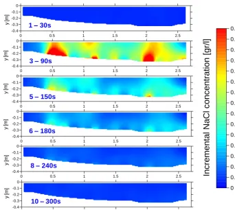
concentration. Such data are reported in Fig. 7, for the same sampling intervals of Fig. 6, and in Fig. 8 in a 3-D representa-tion. The leading edge of the salt plume is clearly evidenced in both images and appears relatively uniform. This suggests that mixing is fairly uniform in early stages. However, at later time intervals, some localized peaks in concentration appear. Particularly in the 3-D interpolation the tailing edges of the plume reveal high concentration zones along the banks of the canal. Because dead zones do not seem to be present in the measuring reach, the results confirm the supposed turbulent but placid flow regime. Indeed the velocity of flow varies from zero at the walls to a maximum in the center, as evi-denced by preliminary qualitative tests using a current meter. This is reflected in the two main concentration peaks located on both sides of the measuring section, and only one of them appears to be correctly sampled by the direct method since the sampling grid has been placed closer to the left down-stream bank (Fig. 3).

By extracting mean and standard deviation values of the concentrations in every tomographic image, it is possible to obtain a trial estimate of the time–concentration curve from geophysical measurements. This interpretation is reported in Fig. 9 and compared to the one obtained from direct mea-surements. As expected, the mass balance of the injected salt extracted from the two evaluations (i.e., multi-sampling sys-tem and cross-flow FERT) differs slightly. The mean values of cross-flow FERT data report a lower concentration peak (approximately 0.1 g L−1_{) with respect to the directly} sam-pled curve.

4 Discussion

3200 C. Comina et al.: Geophysical methods to support correct water sampling locations for salt dilution gauging 25

1

4

3

5

6

0 0.5 1 1.5 2 2.5

-0.4 -0.3 -0.2 -0.1 0

0 0.5 1 1.5 2 2.5

-0.4 -0.3 -0.2 -0.1 0

0 0.5 1 1.5 2 2.5

-0.4 -0.3 -0.2 -0.1 0 -25 -24 -23 -22 -21 -20 -19 -18 -17 -16 -15 -14 -13 -12 -11 -10 -9 -8 -7 -6 -5 -4 -3 -2 -1 0

0 0.5 1 1.5 2 2.5

-0.4 -0.3 -0.2 -0.1 0

0 0.5 1 1.5 2 2.5

-0.4 -0.3 -0.2 -0.1 0

re

s

is

ti

v

it

y

d

if

fe

re

n

c

e

[

o

h

m

.m

]

0 0.5 1 1.5 2 2.5

-0.4 -0.3 -0.2 -0.1 0 x [m] y [m ] y [m ] y [m ] y [m ] y [m ] y [m ]

1 – 30s

3 – 90s

5 – 150s

6 – 180s

8 – 240s

10 – 300s

515

Figure 6. Electric resistivity differences in the imaged section for increasing 516

times (over about 30 s intervals), image number and time indication with reference to 517

Figure 5, seen from up-stream. 518

Figure 6. Electric resistivity differences in the imaged section for increasing times (over about 30 s intervals), image number and time

indication with reference to Fig. 5, seen from upstream.

1. The concentration extracted from cross-flow FERT is an integral concentration over the measuring time, and it takes 30 s (of which 11 s of real acquisition time) to ac-quire the data used in each image. It is therefore pos-sible that part of the plume passing in the measuring section is lost during acquisition. Moreover the mea-suring sequence requires the shifting of the different quadrupoles to different positions along the section dur-ing this time interval which is higher than the one used for direct sampling (5 s). Therefore FERT image inter-pretation will most likely produce a reduced concentra-tion peak value given the speed of the phenomenon un-der observation.

2. The reduced peak concentration observed by cross-flow FERT may also be related to the smoothing of the inver-sion algorithm adopted, which does not allow for vari-ations that are too sharp in conductivity and therefore in concentration. When the concentration distribution within the section is irregular because of spotty and high concentration values, the inverse solution has increased variability. Notably, the larger standard deviation error bars, which, regardless of the statistical distribution of the data, are an index of dispersion around an average

value, are larger near the peak of the plume and smaller towards the end of it.

3. Cross-flow FERT images the whole section of the canal including the left bank zone where there appears to be a reduced concentration area; therefore, with respect to the direct sampling technique, it has the potential to evaluate the entire plume distribution. This results in a more reliable visualization of the plume, and the re-duced concentration peak observed could also be par-tially related to the lower concentration zone near the left bank.

4. The multi-sampling system can be affected by localized high concentration points, which could partially bias to-wards higher concentrations in the overall estimate. In-deed if the maximum concentration value is considered from cross-flow FERT data, the two curves seems to be in better agreement (dashed red line in Fig. 9).

26

0 0.5 1 1.5 2 2.5

-0.4 -0.3 -0.2 -0.1 0

0 0.5 1 1.5 2 2.5

-0.4 -0.3 -0.2 -0.1 0 0 0.01 0.02 0.03 0.04 0.05 0.06 0.07 0.08 0.09 0.1 0.11 0.12 0.13 0.14 0.15

0 0.5 1 1.5 2 2.5

-0.4 -0.3 -0.2 -0.1 0

0 0.5 1 1.5 2 2.5

-0.4 -0.3 -0.2 -0.1 0

0 0.5 1 1.5 2 2.5

-0.4 -0.3 -0.2 -0.1 0

0 0.5 1 1.5 2 2.5

-0.4 -0.3 -0.2 -0.1 0

N

a

C

l

c

o

n

c

e

n

tr

a

ti

o

n

[

g

r/

l]

1 – 30s

3 – 90s

5 – 150s

6 – 180s

8 – 240s

10 – 300s

x [m] y [m ] y [m ] y [m ] y [m ] y [m ] y [m ] 0 0.01 0.02 0.03 0.04 0.05 0.06 0.07 0.08 0.09 0.1 0.11 0.12 0.13 0.14 0.15

In

c

re

m

e

n

ta

l

N

a

C

l

c

o

n

c

e

n

tr

a

ti

o

n

[

g

r/

l]

Figure 7. Concentrations in the imaged section for increasing times (over about 520

30 s intervals), image number and time indication with reference to Figure 5, seen from 521

up-stream. 522

Figure 7. Concentrations in the imaged section for increasing times (over about 30 s intervals), image number and time indication with

reference to Fig. 5, seen from upstream.

Figure 8. 3-D visualization of the passage of the salt plume in the

studied canal section, time axis coherent with Fig. 5.

has been applied, as a function of the cumulative concen-tration for the entire monitored interval, to each point in the imaged section and a representation of discharge vari-ability has been obtained (Fig. 10). Discharge values ob-tained with the above-mentioned process, depicted in Fig. 10,

Figure 9. Comparison of direct sampling and cross-flow FERT

ob-tained concentration curves; the dashed red line refers to the maxi-mum concentration value determined from cross-flow FERT in the area of the canal reported in Fig. 10.

3202 C. Comina et al.: Geophysical methods to support correct water sampling locations for salt dilution gauging

28 531

Figure 10. Discharge variability obtained from the interpretation of FERT 532

compared with the location of direct sampling points (red circles are water spilling 533

tubes). 534

535 536 537

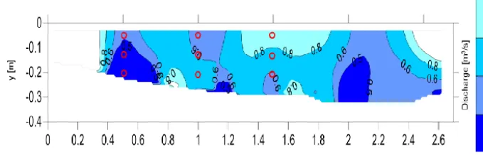
Figure 10. Discharge variability obtained from the interpretation of FERT compared with the location of direct sampling points (red circles

are water spilling tubes).

it can be also observed that some of the spilling tubes ap-pear to be located near low discharge zones (i.e., high con-centration peaks) particularly at the bottom of the canal. In these zones the two estimates appear to be more coherent: lo-cally, areas with 0.5 m3s−1of discharge are evidenced from FERT roughly matching the 0.46 m3s−1 value from direct sampling. The average discharge from direct sampling could be therefore partially biased towards lower values due to the location of the sampling points. The average discharge eval-uated from FERT using only values located in the same posi-tion of the spilling tubes resulted indeed in 0.59 m3s−1, par-tially confirming this hypothesis. It must be also observed that anomalous high discharge values at the bottom of the canal are locally present together with zones on the top of the image in which the too low concentrations observed drive the discharge to unrealistically high values. Even if, due to the flow regime, higher discharge is expected particularly near the free water surface (values around 0.8 m3s−1from FERT), these can be also partially attributed to inverse problem un-certainty and low resolution which, due to the electrodes disposition, is particularly high in the top part of the sec-tion. The quantitative evaluations attempted confirmed that, at present, the FERT technique is a powerful imaging tool but still not completely reliable in estimating an accurate dis-charge value. Only with the development of the technique a space variable quantification of discharge over the testing section could be potentially obtained.

5 Conclusions

Direct sampling of the NaCl (in ionic form) plume from a slug-injection salt dilution test and geophysical imaging of the same salt plume, using cross-flow fast electric resistivity tomography (FERT), have been compared in this work in a single case study. Direct sampling has been performed with a prototype multi-sampling system, obtaining an average value over the sampled area; geophysical data have been acquired and interpreted independently.

The results show that the reconstructed curve from cross-flow FERT seems affected by an overall lower sensitivity

with respect to the peak passage of the plume, and therefore mass balance estimates based on these data cannot be con-sidered completely reliable. At present, the FERT technique still suffers from limitations mainly related to the velocity of acquisition and can therefore only offer qualitative repre-sentations of the salt plume. Nevertheless, cross-flow FERT has provided a reliable visualization of the passage of the plume in the imaged section, showing some localized low-conductivity zones. Because the knowledge of tracer distri-bution in the measuring cross section is very important for the correct placement of sampling points, FERT can be po-tentially used as a preliminary control in this respect. Provid-ing images similar to the ones presented in this study prior to the design of the sampling grid could be very helpful in establishing the most correct direct measurement protocol.

Indeed, discharge measurements by means of the salt dilu-tion method are the most frequently used approaches, espe-cially in difficult-to-access areas: in these situations, testing requirements are often not easily accomplished due to logis-tical conditions. It is also not always easy to establish a priori whether all the test requirements are satisfied.

Geophysical imaging can therefore be an important aid offering a direct visualization of the salt plume and conse-quently a more precise location of sampling points. Follow-ing this first visualization, a samplFollow-ing optimization in the downstream sampling section, using a multi-sampling tech-nique, is strongly recommended. Sampling the canal water in different points of a cross section, by means of simultaneous water picking up, can optimize the quantitative detection and results in more reliable discharge estimates.

Acknowledgements. This research has been partially funded

in the framework of a research project between the Agricul-tural Management of Piedmont Region and the Earth Science Department of Università degli Studi di Torino. Authors are indebted with Paolo Clemente, Giovanna Dino, Diego Franco, Francesco Marzano and Sabrina Bonetto for their help in the execution of the field tests.

Edited by: A. D. Reeves

References

Clemente, P., De Luca, D. A., Dino, G. A., and Lasagna, M.: Wa-ter losses from irrigation canals evaluation: comparison among different methodologies, Geophys. Res. Abstr., EGU2013-9024, EGU General Assembly 2013, Vienna, Austria, 2013.

Drost, J. W.: Single-Well and Multi-Well Nuclear Tracer Tech-niques – a Critical Review, Technical Documents in Hydrol-ogy, International Hydrological Programme 96, UNESCO, Paris, 1989.

Fangary, Y. S., Williams, R. A., Neil, W. A., Bond, J., and Faulks, I.: Application of electric resistance tomography to detect de-position in hydraulic conveying systems, Powder Technol., 95, 61–66, 1998.

Gees, A.: Flow measurement under difficult measuring conditions: Field experience with the salt dilution method, in: Hydrology in Mountainous Regions I. Hydrological Measurements; The Water Cycle, edited by: Lang, H. and Musy, A., IAHS Publ., 193, 255– 262, 1990.

Hudson, R. and Fraser, J.: Alternative methods of flow rating in small coastal streams, Extension Note EN-014 Hydrology, Van-couver Forest Region, B.C. Ministry of Forests, VanVan-couver, p. 11, 2002.

Jaramillo, F.: Estimating and modeling soil loss and sediment yield in the Maracas-St. Joseph River Catchment with empirical mod-els (RUSLE and MUSLE) and a physically based model (Ero-sion 3D), Master in Civil Engineering-Thesis, McGill University, Montreal, 134 pp., 2007.

Kite, G.: Computerized streamflow measurement using slug injec-tion, Hydrol. Process., 7, 227–233, 1993.

Kumar, B. and Nachiappan, R. P.: Estimation of alluvial aquifer pa-rameters by a single-well dilution technique using isotopic and chemical tracers: a comparison, in: Tracers and Modelling in Hy-drogeology, IAHS Publ. 262, edited by: Dassargues, A., IAHS Press, Wallingford, 53–56, 2000.

Lucas, G. P., Cory, J., Waterfall, R. C., Loh, W. W., and Dickin, F. J.: Measurement of the solids volume fraction and velocity distribu-tions in solids–liquid flows using dual-plane electrical resistance tomography, Flow Meas. Instrum., 10, 249–258, 1999.

Moore, R. D.: Introduction to salt dilution gauging for streamflow measurement: Part I, Streaml. Watershed Manage. Bull., 7, 20– 23, 2004.

Moore, R. D.: Slug injection using salt in solution, Streaml. Water-shed Manage. Bull., 8, 1–6, 2005.

Perotti, L., Clemente, P., De Luca, D. A., Dino, G. A., and Lasagna, M.: Remote sensing and hydrogeological methodologies for ir-rigation canal leakage detection: the Osasco and Fossano test sites (Northwestern Italy), Geophys. Res. Abstr., EGU2013-5705, EGU General Assembly 2013, Vienna, Austria, 2013. Radulovic, M., Radojevic, D., Devic, D., and Blecic, M.:

Dis-charge calculation of the spring using salt dilution method – application site Bolje Sestre Spring (Montenegro), avail-able at: http:25//balwois.com/balwois/administration/fullpaper/ ffp-1257.pdf (last access: 24 July 2013), 2008.

Rantz, S. E.: Measurement and Computation of Streamflow: Vol-ume 1. Measurement of Stage and Discharge, US Geological Survey Water-Supply Paper 2175, US Department of the Interior, US Government Printing Office, Washington, D.C., 1982. Sambuelli, L. and Comina, C.: Fast ert to estimate pollutants and

solid transport variation in water flow: a laboratory experiment, B. Geofis. Teor. Appl., 51, 1–22, 2010.

Sambuelli, L., Lollino, G., Morelli, G., Socco, L. V., and Bidone, L.: First experiments on solid transport estimation in river-flow by fast impedance tomography, VIII EEGS meeting, 8–15 Septem-ber, Aveiro, Portugal, 4 pp., 2002.

Scobey, F. C.: Flow of water in irrigation and similar canals, US Dept. of Agriculture, Washington, D.C., 79 pp., 1939. Tapp, H. S. and Wilson, R. H.: Developments in low-cost electrical

imaging techniques, Process Contr. Qual., 9, 7–16, 1997. Tazioli, A.: Experimental methods for river discharge

measure-ments: comparison among tracers and current meter, Hydrolog. Sci. J., 56, 1314–1324, 2011.

Wang, M. and Cilliers, J. J.: Detecting non-uniform foam den-sity using electrical resistance tomography, Chem. Eng. Sci., 54, 707–712, 1999.

Warsito, W. and Fan, L. S.: Measurement of real-time flow struc-tures in gas–liquid and gas–liquid–solid flow systems using electrical capacitance tomography (ECT), Chem. Eng. Sci., 56, 6455–6462, 2001.

Xie, C. G., Reinecke, N., Beck, M. S., Mewes, D., and Williams, R. A.: Electrical tomography techniques for process engineering applications, Chem. Eng. J., 56, 127–133, 1995.

Yang, W. Q. and Liu, S.: Role of tomography in gas/solids flow measurement, Flow Meas. Instrum., 11, 237–244, 2000. Zellweger, G. W.: Testing and comparison of four ionic tracers to