Hydrol. Earth Syst. Sci., 12, 989–1006, 2008 www.hydrol-earth-syst-sci.net/12/989/2008/ © Author(s) 2008. This work is distributed under the Creative Commons Attribution 3.0 License.
Hydrology and
Earth System
Sciences
HYDROGEIOS: a semi-distributed GIS-based hydrological model
for modified river basins
A. Efstratiadis1, I. Nalbantis2, A. Koukouvinos1, E. Rozos1, and D. Koutsoyiannis1
1Department of Water Resources and Environment, School of Civil Engineering, National Technical Univ. of Athens, Greece 2Laboratory of Reclamation Works and Water Resources Management, School of Rural and Surveying Engineering, National Technical Univ. of Athens, Greece
Received: 15 June 2007 – Published in Hydrol. Earth Syst. Sci. Discuss.: 28 June 2007 Revised: 16 May 2008 – Accepted: 26 June 2008 – Published: 28 July 2008
Abstract. The HYDROGEIOS modelling framework
repre-sents the main processes of the hydrological cycle in heavily modified catchments, with decision-depended abstractions and interactions between surface and groundwater flows. A semi-distributed approach and a monthly simulation time step are adopted, which are sufficient for water resources management studies. The modelling philosophy aims to en-sure consistency with the physical characteristics of the sys-tem, while keeping the number of parameters as low as pos-sible. Therefore, multiple levels of schematization and pa-rameterization are adopted, by combining multiple levels of geographical data. To optimally allocate human abstractions from the hydrosystem during a planning horizon or even to mimic the allocation occurred in a past period (e.g. the calibration period), in the absence of measured data, a lin-ear programming problem is formulated and solved within each time step. With this technique the fluxes across the hy-drosystem are estimated, and the satisfaction of physical and operational constraints is ensured. The model framework includes a parameter estimation module that involves vari-ous goodness-of-fit measures and state-of-the-art evolution-ary algorithms for global and multiobjective optimization. By means of a challenging case study, the paper discusses appropriate modelling strategies which take advantage of the above framework, with the purpose to ensure a robust cali-bration and reproduce natural and human induced processes in the catchment as faithfully as possible.
Correspondence to: A. Efstratiadis
1 Introduction
system, especially in leaky basins, with complex interac-tions between soil and aquifer. Besides, detailed historical data regarding abstractions are usually missing, especially when these are implemented through small private works (e.g. wells). Therefore, additional modelling is required to estimate abstractions, on the basis of theoretical water de-mands.
In the last years, several approaches have appeared on cou-pling hydrological models for surface and sub-surface flows (e.g., Singh and Bhallamudi, 1998; Panday and Huyacorn, 2004). Typically, however, these approaches do not repre-sent all aspects of an operational water management prob-lem at the river basin scale. Moreover, they preclude us-ing stochastic simulation and forecastus-ing, which are effi-cient methods to support water management. On the other hand, in most decision support systems (DSSs) for water resources management water flows are represented through network-type hydrosystems, thus ignoring the distributed regime of hydrological processes. In some cases, the prob-lem is tackled by means of special eprob-lements in the hydrosys-tem, based on some form of elementary lumped models, such as the “groundwater reservoir node” in the RIBASIM software (Waterloopkundig Laboratorium, 1991). However, these elements, apart from being too simplified, contain pa-rameters that normally require calibration (Nalbantis et al., 2002). Attempts to bridge this gap are very few, such as the MODSIM package (Fredericks et al., 1998; Dai and Labadie, 2001).
HYDROGEIOS is a new, GIS-based software system that provides a holistic framework, aiming at combining hydro-logical and hydrogeohydro-logical simulation in modified basins. The model represents the governing interactions between surface flows, groundwater flows and man-made interven-tions, on the basis of a semi-distributed configuration. It integrates ideas from previous approaches (Nalbantis et al., 2002; Rozos et al., 2004; Rozos and Koutsoyiannis, 2006), whereas some components (e.g. the GIS module) are en-tirely new. HYDROGEIOS uses historical hydrological data for calibration and validation, as well as synthetic data for stochastic forecasting; in the last case, it co-operates with the DSS HYDRONOMEAS, which implements the optimization of the hydrosystem operation policy (Koutsoyiannis et al., 2002; Koutsoyiannis et al., 2003; Efstratiadis et al., 2004). Regarding the conceptualization, model parameters retain some physical consistency, since they are assigned on the basis of distributed data. For their estimation, the software encompasses a specific module, containing multiple fitting measures, statistical and empirical, and evolutionary algo-rithms for single-objective and multiobjective optimization.
2 Parameter uncertainty and calibration
Uncertainty is an inherent characteristic of all hydrological processes, further amplified by the weaknesses of
determin-istic conceptual watershed models, whose parameters are es-timated through calibration. Uncertainty is due to system complexity and multiple error sources, which are interact-ing in an unknown manner, thus makinteract-ing the traditional au-tomatic calibration approach behave like a black-box math-ematical game. Apart from evident errors in raw measure-ments and data-processing, typical sources of uncertainty are the inadequate representation of processes or, in the oppo-site, the formulation of too complex representations, unable to be supported by the existing knowledge about the physi-cal system (Refsgaard, 1997; Wagener et al., 2001; Butts et al., 2004), the poor representation of the temporal and spatial variability of model forcing (Paturel et al., 1995; Chaubey et al., 1999; Beven, 2000; Andr´eassian et al., 2001), the non-representativeness of calibration data and the use of statis-tically inconsistent fitting criteria (Sorooshian and Dracup, 1980; Kuczera, 1982; Sorooshian et al., 1983; Yapo et al., 1996; Gan et al., 1997), the poor identification of initial and boundary conditions (Kitanidis and Bras, 1980), the weak-nesses of most optimization methods to handle response sur-faces of irregular topography (Duan et al., 1992), as well as the temporal changes of natural and anthropogenic processes (Nandakumar and Mein, 1997; Brath et al., 2006; Ewen et al., 2006). The above problems have been thoroughly exam-ined for more than three decades, concluding that uncertainty is inherent, thus unavoidable, and increases with model com-plexity. Uncertainty is also strongly related to the “equifinal-ity” concept (Beven and Binley, 1992), practically identified as the existence of multiple acceptable parameter sets, on the basis of different model configurations, calibration data and fitting criteria. As a consequence of equifinality, it is im-possible to detect a “global” optimal model structure or a “global” optimal parameter set, which definitely better re-produce the entire hydrological regime of a river basin.
In the last years, a variety of mathematical techniques were developed to quantify the uncertainty of conceptual model predictions. Most of them are embedded in the calibration procedure and seek “promising” trajectories of model out-puts that correspond to multiple, “behavioural” parameter sets (Beven and Binley, 1992; Freer et al., 1996; Kuczera and Parent, 1998; Thiemann et al., 2001; Vrugt et al., 2002). Yet, their application indicates that, usually, the model predictive uncertainty proves comparable to the statistical uncertainty of the measured outputs. Moreover, many questions arise re-garding the practical aspects of uncertainty analysis methods, such as the computational effort for multidimensional appli-cations, the acceptance by policy makers and the public, and the inability to provide a final decision regarding a unique “best-compromise” parameter set (Pappenberger and Beven, 2006).
A. Efstratiadis et al.: HYDROGEIOS: a semi-distributed model for modified basins 991 2001). This is the reason why many researchers tend to
em-ploy optimization for a small portion of the parameters (Refs-gaard, 1997; Beven, 2001; Eckhardt and Arnold, 2001; Mad-sen, 2003; Vrugt et al., 2004; Muleta and Nicklow, 2005). In any case, integrating physically-based schemes within river basin management models has severe practical drawbacks, regarding the amount of spatial data required and the pro-hibitive computational effort.
Recent research revealed the advantages of conceptual semi-distributed models for streamflow estimation, in com-parison to lumped ones (Boyle et al., 2001; Ajami et al., 2004). Such schemes allow a satisfactory representation of watershed heterogeneities, provide the required level of de-tail for an engineering application (due to the network-type configuration), while being computationally efficient. How-ever, if interior calibration data are missing (e.g., hydro-graphs across the river basin), any movement from a lumped to a semi-distributed approach increases model complexity which, in turn, creates more uncertainty in the results.
HYDROGEIOS employs a semi-distributed scheme for the spatial representation of physical processes in modified hydrosystems. Instead of allocating parameters per sub-basin, the parameterization of surface hydrological processes is implemented on the basis of hydrological response units (HRUs). The term was introduced by Fl¨ugel (1995) to char-acterize homogeneous areas with similar geomorphologic and hydrodynamic properties. The concept is widely used in distributed models, such as SWAT (Srinivasan et al., 2000), where the river basin is assumed to be an assembly of dis-crete entities with different characteristics that contribute dif-ferently to its responses. While a HRU is defined to serve a particular model conceptualization, commonly it denotes a spatial element of pre-determined geometry, identical to the schematization of the watershed. The main drawback of this approach is the huge number of unknown properties involved, which may be two or three orders of magnitude larger than the number of parameters of a lumped model, as indicated by Refsgaard (1997). To handle this problem in HYDROGEIOS, the HRU concept is used differently; it rep-resents soil and land types, defining partitions of the basin, rather than “units” of contiguous geographical areas. In ticular, the HRUs are defined as the product of separate par-titions accounting for different properties such as soil per-meability, land cover, terrain slope, etc. This product is for-mally known as common refinement of the partitions, while in the GIS terminology the related procedure is often called “union of layers”. Through an appropriate classification of the above properties, one can adjust the number of HRUs and, consequently, the number of the parameters describing the soil hydrological mechanisms. Hence, parameters retain some physical meaning, which also allows a better identi-fication of their prior uncertainty (i.e., the lower and upper bounds, used in calibration). Similar to surface water pro-cesses, the groundwater processes are represented through discretising the aquifer, by means of polygonal cells. There
are no specific restrictions in the shape of cells, contrary to the majority of groundwater models, which implement a de-tailed, grid-based schematization.
The flexibility in the definition of the HRUs and the multi-cell representation of the aquifer allows the formulation of modelling schemes of variable complexity, depending on the available geographical and input data and the desirable pa-rameterization. In contrast, the schematization of the hy-drosystem, regarding the configuration of the physical and artificial network, is only restricted by the specified study re-quirements (i.e. the location of control points for the water balance calculations), and has no practical influence on the number of parameters. This is consistent with the principle of parsimony, which stands as a key point to handle uncer-tainties in model predictions. The simplest schematization and parameterization is ensured by using as many degrees of freedom as can be explained by the available “knowledge” about the system, regarding the hydrological and geographi-cal data as well as the modeller’s experience.
Results from previous research suggest that only five or six parameters can be identified on the basis of a single hy-drograph (Jakeman and Hornberger, 1993); otherwise, pa-rameter uncertainty due to poor identifiability may limit sig-nificantly the predictive capacity of models (Wagener et al., 2001). Thus, apart from a parsimonious configuration, it is critical to increase the amount of information in calibration, using multiple output variables and multiple performance measures, since a single measure would likely fail to repro-duce all essential characteristics of the physical system that are reflected in the observations (Gupta et al., 1998).
3 Model overview
3.1 Model formulation and input data
Since HYDROGEIOS is focused on the water resources management problem, the entire modelling approach is based on a network-type schematization of the physical and the artificial components of the hydrosystem. The two net-works are linked together through water diversions, abstrac-tions and disposals. The aquifer is also modelled as a net-work of conceptual storage (tanks) and transportation ele-ments (conduits) connecting adjacent tanks. Most compo-nents have georeference and are handled through a GIS mod-ule, implemented in an ArcGIS environment. This module is also used for processing distributed data, used in the formula-tion of the HRUs, and the generaformula-tion of the derivative layers (unions, intersections).
3.1.1 Hydrographic network
The schematization of the hydrographic network is imple-mented through a two-step procedure. First, an initial net-work is formulated on the basis of a digital terrain model, by adjusting the flow accumulation parameter. Next, additional control points are added across the network, which corre-spond to flow monitoring stations, abstraction points, inflow nodes, etc. The sub-basins upstream of each node are then created such that each river segment crosses a unique sub-basin.
Hydrological inputs are precipitation and potential evap-otranspiration time series, assigned to each sub-basin. For each sub-basin, the model calculates the transformation of precipitation to actual evapotranspiration, deep percolation and surface runoff; the latter is transferred as point inflow to the corresponding downstream node. The related processes are conceptualized via the soil moisture accounting model, described in Sect. 3.2.1. All calculations are implemented on a derivative layer, generated as the product of the sub-basin and HRU layers, since meteorological forcing (precipitation and potential evapotranspiration) varies for each sub-basin. 3.1.2 Water management network
The applicability of HYDROGEIOS to modified basins is ensured through a coarse depiction of the major hydraulic works (pipes, channels, wells, etc.), the corresponding water uses and constraints and their interactions with the physical system. All are represented as network components, namely nodes and aqueducts; the latter may conduct water to the hy-drographic network or abstract it to satisfy demands. Finally, wells lying on neighbouring locations and serving the same use are conceptualized as clusters, named borehole groups.
The network properties are discharge and pumping capaci-ties, target prioricapaci-ties, demand time series and unit transporta-tion costs. The priorities and costs are assigned to express preferences regarding the allocation of abstractions, in case
of multiple water sources and conveyance paths. When a de-mand can be fulfilled through different abstractions, the user can impose unit costs (actual or hypothetical ones) to the cor-responding aqueducts. For instance, a zero and a positive unit cost for surface and groundwater abstractions, respectively, will force the model to abstract water from the river rather than from groundwater. The preservation of target priorities and the minimization of costs are both ensured via the flow allocation model, explained in Sect. 3.2.3.
3.1.3 Groundwater network
The aquifer is represented as a multicell network, on the ba-sis of a polygonal discretization of the aquifer. According to Rozos and Koutsoyiannis (2005), the mathematical concept derives from the finite volume method, provided that the cell edges are parallel or normal to the equipotential contours and the line joining the centroids of adjacent cells is perpendic-ular to their common edge. This approach enables the ex-ploitation of the available piezometric data for the study area. Moreover, the flexible number and shape of cells allows the description of aquifers of complex geometries on the basis of the physical characteristics of the system (e.g., geology) through parsimonious structures. Hence, the parameteriza-tion has a physical concept and the computaparameteriza-tional effort is significantly reduced, when compared to typical finite differ-ence or finite element schemes.
Input properties are the top and bottom elevation of each tank and the water table at the beginning of simulation (ini-tial condition of the model). Regarding boundary conditions, the user can prohibit the exchange of water between neigh-bouring cells, assuming an impervious common edge. The geometrical properties are automatically computed via the GIS module. These include cell areas, centroid coordinates, distances and common edge lengths between adjacent cells, plus all unions and intersections with the surface geographi-cal layers. Note that some cells may lie out of the watershed bounds, to direct the groundwater sinks to the sea or neigh-bouring basins. Other components are springs, which rep-resent point outflows that are transferred to the downstream node of the corresponding sub-basin; their properties are the altitude and the interconnected cell.
3.2 Mathematical framework
The mathematical representation of the hydrological, hydro-geological and anthropogenic processes is based on the com-bination of three related models running within a loop, as explained in Sect. 3.2.4. The time scale of simulation is monthly, which is sufficient for water management studies. 3.2.1 Surface hydrology model
A. Efstratiadis et al.: HYDROGEIOS: a semi-distributed model for modified basins 993 scheme, illustrated in Fig. 1. Model inputs are the areal
pre-cipitationPtand potential evapotranspirationEP t, while
out-puts are the soil moistureSt, the surface runoffQt, the actual
evapotranspirationEt, and the percolationGt. At each time
stept, the water balance equation is written in the form:
St+1=St+Pt−Qt−Et−Gt (1)
For a given value of soil storage at the beginning of simu-lation, the above formula is solved on the basis of some as-sumptions regarding the unknown variablesQt,EtandGt.
The ground operates as a filter, transforming precipitation to direct evapotranspirationEDt, direct runoffQDt, and
infil-trationIt. Direct evapotranspiration represents the amount of
precipitation evaporated quickly, before infiltrating, and can-not exceed a retention capacityR, and the theoretical demand EP t. Direct runoff represents the excess of precipitation
con-ducted through the impervious areas of the basin to its outlet within the time interval, and calculated asQDt=c(Pt−EDt),
wherecis a constant ratio that depends on the physical prop-erties of the ground (soil permeability, vegetation, slope) and the existence of flood-prevention works.
The remaining precipitation infiltrates to the unsaturated zone, represented as a soil moisture accounting tank of ca-pacity Smax. The tank is divided into two zones (upper and lower), using a dimensionless parameterκ. The evap-otranspiration deficit, i.e. the amountEP t−EDt, is satisfied
by the actual moisture, using different mechanisms for the two zones. Specifically, the whole amount of moisture in the upper zone is assumed available for evapotranspiration, whereas the lower zone moisture is partially available. In the last case, the rate of soil evapotranspiration is taken to be pro-portional to the ratioSLt/(κSmax), whereSLt is the moisture
depth stored in the lower zone andκSmaxis the correspond-ing capacity. The process is mathematically expressed by a declining exponential function, similar to that of the well-known Thornthwaite model (Thornthwaite, 1948).
Moreover, the soil moisture tank provides options for hori-zontal and vertical outflow, implemented via two orifices, the one lying at levelκSmaxand the other at the bottom. These represent a time-lagged runoff component (interflow) QI t
and the percolation to deeper zonesGt, respectively. The
corresponding outflow rates are controlled through the reten-tion coefficientsλandµ.
At the end of the simulation step, the soil moisture excess (if it exists) contributes to the streamflow as quick runoff due to saturation, QSt. Within the time interval the storage is
allowed to exceedSmax.
Model parameters are the retention capacityR, the direct runoff coefficientc, the soil capacitySmax, the ratio of the lower zone capacity to the total one κ, and the retention coefficientsλ,µfor interflow and percolation, respectively. These differ for each HRU, as explained in Sect. 3.1.1. All variables are integrated to the sub-basin scale, except for the percolation, which is integrated to the groundwater cell scale. The model then adds to the surface flow, the direct, quick and
37
ES = ESU+ ESL
P
G = µ S
QS
QI= λ(S -SL)
SL= κSmax
Smax S
QD= c (P–ΕD)
Q ED = min (P, R, EP)
Ι= P–ED –QD
E
EP
Precipitation
Percolation Direct runoff
Saturation runoff
Interflow Evapotranspiration
from upper and lower zone
Direct (ground)
evapotranspiration Infiltration Potential evapotranspiration
Moisture storage
Interception
Upper zone
Lower zone Soil
capacity
Figure 1: Schematic layout of the surface water balance model.
Surface hydrology model
Groundwater model
Water management model
Percolation
Spring runoff & sea losses
Pu
m
pin
g &
ri
ver
in
fi
ltra
ti
on
Surface runoff
Water balance (flows & abstractions) Water
needs
Precipitation
Surface hydrology model
Groundwater model
Water management model
Percolation
Spring runoff & sea losses
Pu
m
pin
g &
ri
ver
in
fi
ltra
ti
on
Surface runoff
Water balance (flows & abstractions) Water
needs
Precipitation
Figure 2: Simulation flowchart, explaining the interaction of the three models.
Fig. 1. Schematic layout of the surface water balance model.
time-lagged runoff components, and the baseflow arriving from the springs located in the sub-basin. A percentage of the total runoff, equal to an infiltration coefficientδassigned to each river segment crossing the sub-basin, recharges the groundwater system, whereas the rest is conducted to the outlet node, as point inflow to the hydrographic network; the coefficientδis either pre-specified or estimated through cal-ibration.
3.2.2 Groundwater model
Each groundwater cell is represented by a conceptual tank, whose parameters are the specific yield (dimensionless) and the conductivity, expressed in velocity units. The stress com-ponents of groundwater tanks are: (a) areal inflows due to percolation through each sub-basin and HRU combination; (b) inflows due to infiltration underneath each river segment; and (c) point outflows due to pumping from each well.
We remind that percolation rates are output of the sur-face hydrological model, whereas infiltration and pumping rates are output of the water management model. Regarding percolation, the model integrates the equivalent depths from each sub-basin and HRU combination on the corresponding cell area. Regarding infiltration, the model estimates the river segment losses supplying each tank, assuming that:
Iij =IjLij/Lj (2)
whereIj is the sum of infiltration losses through the river
segmentj, Lj is the segment length and Lij is its partial
length over celli.
as follows: hi =
nwmin
i + wi wi ≤bi
wimax+(wi −bi)θ wi > bi
(3)
wherewi is the water level in tanki,wiminandwmaxi are the
bottom and top absolute levels, respectively (wmaxi =wmini + bi),θ is the ratio of specific yield to confined storage
coef-ficient andbi is the layer thickness. The upper equation in
(3) corresponds to phreatic conditions, while the lower cor-responds to confined conditions, so thatbirepresents also the
threshold between confined and unconfined conditions. The water volume contained in the tank equals the base area of the corresponding cell multiplied by the level and the spe-cific yield; a low value of the latter indicates that a large wa-ter level increase is required to store a particular amount of groundwater, and vice versa.
A constant head condition is represented by assigning tanks with very large base, which forces the corresponding water level to remain practically constant and close to the prescribed boundary value. Likewise, springs are modelled assuming such dummy tanks, for which the slight changes of the water level are directly transformed into outflow hydro-graphs. A similar representation is implemented for simulat-ing groundwater losses, conducted to neighboursimulat-ing basins or the sea.
Groundwater flows are implemented through conceptual conduits (i,j), where the indices denote the interconnected tanks. Their properties are the cross sectional areaAij(equal
to the common plane area between cellsi andj, which is assumed constant within each time interval), the lengthlij
(centroid distance) and the conductivity Kij, computed as
the arithmetic or geometrical mean of the corresponding tank conductivities. The dischargeQij is calculated using a
Dar-cian formula: Qij =KijAij
hi−hj
lij
(4) wherehi andhj are the head values of the adjacent tanksi
andj.
Equations (3) and (4) formulate a system of equations that can be solved via explicit or implicit numerical schemes. HYDROGEIOS implements both schemes, for which a proper time discretization (i.e. number of time intervals within a simulation step) must be defined, to ensure numeri-cal stability.
3.2.3 Water management model
Outputs of the surface and groundwater hydrological models are the sub-basin and spring runoff, both assumed as point inflows to the river network. The water allocation is imple-mented on the unified network, to define the unknown fluxes through the entire hydrosystem. These include the discharge rates and losses (due to leakage) across the river and the
aquifer and, subsequently, the abstractions from surface and groundwater resources.
The modelling concept is based on a linear programming (LP) approach. Similar ones have been used in some water resource planning and management applications, where lin-ear optimization is embedded within simulation to find the least cost flow allocation through hydrosystems of network format (Graham et al., 1986; Kuczera, 1989; Fredericks et al., 1998; Dai and Labadie, 2001). The optimization is based on real economic criteria or artificial costs, assigned to pre-serve water rights and water use priorities.
HYDROGEIOS implements a simplified version of the scheme described by Efstratiadis et al. (2004). The gen-eral idea is to distinguish the hydrosystem variables and op-timally allocate them through the hydrosystem, which is rep-resented as a digraph. Apart from real world components, the digraph includes dummy nodes and links where virtual attributes are imposed, namely the conveyance capacity and the unit transportation cost. The latter may be either posi-tive or negaposi-tive. Particularly, posiposi-tive unit costs are imposed to penalize non-desirable water fluxes, whereas negative unit costs are imposed to force the model to provide water to fulfil the physical and operational constraints. Specifically:
– Leaky river segments are represented by two links, the
one carrying the discharge arriving at the downstream node, and the other carrying the infiltration, which is transferred to an accounting node, a fictitious compo-nent inserted for mathematical convenience (to ensure that the sum of inflows equals the sum of outflows).
– River segments or aqueducts, where minimum flow
preservation targets are imposed, are represented by two parallel links, the one having discharge capacity equal to the actual target value and negative cost, whereas the other has the rest of capacity (infinite in the case of a river segment) and unit cost equal to the real transporta-tion cost (zero in case of river segment). Maximum flow targets are handled in the same way; positive cost is used here to prevent the violation of the discharge bound.
– Borehole groups are represented through a virtual
groundwater node, the inflow of which is equal to the total pumping capacity of the wells. Two links are con-nected to this node, the one carrying the groundwater abstraction to the corresponding downstream node with unit cost equal to the total pumping charge, and the other transferring the rest of inflow to the accounting node, without cost.
– Demand nodes are connected with the accounting node
A. Efstratiadis et al.: HYDROGEIOS: a semi-distributed model for modified basins 995 The transformation of hydrosystem components to digraph
components and the assignment of capacity and unit cost val-ues are automatically executed by the program. Most for-mulations are done once, at the beginning of each simula-tion. Especially, the assignment of costs is a key part of the model, since this ensures the preservation of both feasibility and economy. Feasibility refers to the strict satisfaction of all physical constraints (nodal water balance equations and arc capacity bounds) and the hierarchical satisfaction of water uses, keeping the user-defined priorities, whereas economy refers to the minimization of total transportation and pump-ing costs.
The problem is expressed as: minimizef (x)=cTx
subject to Ax=y
1x=0
0≤x≤u (5)
wherexis the vector of control variables, corresponding to the hydrosystem fluxes;cis the vector of unit costs; A is the incidence matrix, describing the continuity equations, with elements taking values{−1, 1, 0};1is a matrix describing constraints for leaky segments, with elements taking values {−1,δi/(1−δi), 0}; y is the vector of inflows; anduis the
vector of link capacities. Due to the particular structure of (5), primarily the sparse format of matrix A, its solution is very fast through appropriate versions of the simplex method, thus ensuring computational efficiency.
3.3 Model integration within simulation
Due to the interactions between surface and groundwater re-sources, as well as the physical and man-made processes, the application of the aforementioned models within simulation requires a looped architecture, as illustrated in Fig. 2. At the beginning of each time step, dynamic input data includes pre-cipitation and potential evapotranspiration depths, assigned at each sub-basin, and water demand values, assigned at spe-cific nodes of the hydrosystem. The remaining hydrological variables are unknown, and for some of them initial guesses are necessary. The simulation procedure is implemented as follows:
First, and outside of the loop, the surface hydrological model runs to estimate real evapotranspiration, percolation, surface runoff and soil moisture for each combination of sub-basins and HRUs. Runoff is transferred to the outlet node of each sub-basin, after adding baseflow and, then, excluding losses due to infiltration. Baseflow is computed by adding discharge values of springs lying in each sub-basin. Initially, these are assumed equal to the values of the previous time step, but as the loop proceeds, the real ones are assigned, as estimated from the groundwater model.
Next, the water management scheme runs to estimate all hydrosystem fluxes, i.e. discharge and infiltration
val-37
ES = ESU+ ESL
P
G = µ S
QS
QI= λ(S -SL)
SL= κSmax
Smax S
QD= c (P–ΕD)
Q
ED = min (P, R, EP)
Ι= P–ED –QD E
EP
Precipitation
Percolation Direct runoff
Saturation runoff
Interflow Evapotranspiration
from upper and lower zone
Direct (ground)
evapotranspiration Infiltration
Potential evapotranspiration
Moisture storage
Interception
Upper zone
Lower zone Soil
capacity
Figure 1: Schematic layout of the surface water balance model.
Surface hydrology model
Groundwater model
Water management model
Percolation
Spring runoff & sea losses
Pu
m
pin
g &
ri
ver
in
fi
ltra
ti
on
Surface runoff
Water balance (flows & abstractions) Water
needs
Precipitation
Surface hydrology model
Groundwater model
Water management model
Percolation
Spring runoff & sea losses
Pu
m
pin
g &
ri
ver
in
fi
ltra
ti
on
Surface runoff
Water balance (flows & abstractions) Water
needs
Precipitation
Figure 2: Simulation flowchart, explaining the interaction of the three models. Fig. 2. Simulation flowchart, explaining the interaction of the three
models.
ues across the hydrographic network, and abstractions from surface and groundwater resources. Inflows to the digraph model are runoff values, assigned downstream of each sub-basin, already known from the surface hydrological model, as well as external inflows, given as known time series.
The implementation of the above models allows the as-signment of groundwater stresses at each cell. These are es-timated by adding percolation from each sub-basin and HRU combination and infiltration from each river segment, and ex-cluding pumping from each well. Next, the groundwater flow model is solved, to estimate the tank levels, the spring flows and the underground losses.
Based on the actual evaluation of spring discharge, HY-DROGEIOS recalculates baseflow and corrects all runoff es-timates. This requires new runs of the water management and groundwater models, until stabilization of baseflow. Practi-cally, this scheme converges after one or two cycles only, thus ensuring both accuracy and efficiency.
4 Calibration framework
4.1 Fitting measures
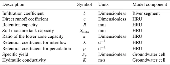
Table 1. List of model parameters.
Description Symbol Units Model component
Infiltration coefficient δ Dimensionless River segment Direct runoff coefficient c Dimensionless HRU
Retention capacity R mm HRU
Soil moisture tank capacity Smax mm HRU
Ratio of the lower zone capacity κ Dimensionless HRU Retention coefficient for interflow λ d−1 HRU Retention coefficient for percolation µ d−1 HRU
Specific yield Sy Dimensionless Groundwater cell
Hydraulic conductivity K m/s Groundwater cell
parsimony. In accordance with this, HYDROGEIOS pro-vides a set of statistical and empirical fitting measures for the calibration of parameters, to control the observed out-puts as well as the internal state variables of the groundwater model (i.e. tank levels). The criteria are aggregated to one or more weighted objective functions, to determine a single or multiple (i.e. non-dominated) optimal parameter sets.
The statistical measures used are the coefficient of effi-ciency, also known among hydrologists as the Nash-Sutcliffe index (Nash and Sutcliffe, 1970), and the bias in the mean, the standard deviation and the coefficient of variation of mea-sured responses; the latter may refer to both discharge and level time series. Yet, due to the usually rough delineation of the groundwater field, resulting to large cell areas and thus relatively small variability of the corresponding simulated levels, one should employ very carefully calibration on the basis of observed water table data, due to the issue of scale compatibility.
Furthermore, the model uses an empirical penalty term, to better control the intermittencies, since a “zero discharge” state is very frequent, and its reproduction is important for a water management study. Given the observed and simulated time series,yt andyt0, respectively, the penalty is calculated
as:
e0= v u u t 1 T0
T
X
t=1
zt2 (6)
whereztis an auxiliary variable, computed as:
zt =
(y
t ifyt0=0
yt0ifyt=0
0 else
(7)
andT0the number of time steps for which the model fails to reproduce an observed flow interruption or, in the opposite, erroneously yields zero discharge.
A final measure is used to control the behaviour of the internal model variables, specifically the generation of un-reasonable trends regarding groundwater levels, based on the
Mann-Kendall rank correlation test (Kottegoda, 1980, p. 32– 34). When attempting to calibrate the groundwater parame-ters (i.e., conductivities) merely on spring hydrographs, with-out using observed level data, a conjunctive model could eas-ily preserve the water balance of surface flows by leaving some upstream tanks empty and, simultaneously, accumu-lating the excess of water downstream. This situation is not consistent with the physical behaviour of an aquifer, the level of which follows the typical seasonal and overyear fluctua-tion of precipitafluctua-tion. However, in heavily modified basins with intensive exploitation of groundwater, a systematic de-cline of the water table could occur. Thus, even if level data is totally missing, an appropriate use of the trend penalty should significantly improve the identifiability of the ground-water parameters, thus leading to more reliable schemes.
The Mann-Kendall test is implemented as follows: Given a sample (x1,x2, ...,xN), the statisticT=r/
p σ2
r is a standard
normal variable, where:
r=4P /[N (N−1)], σr2=2(2N+5)/[9N (N−1)] (8) andP is the number of all pairs{xi,xj,j >i}withxi<xj.
For a two-tailed test and for a level of significance a, we reject the null hypothesis of no trend presence if|T|<za/2. In that case, a penalty value equal to|T|−za/2is assigned. 4.2 Optimization algorithms
4.2.1 The evolutionary annealing-simplex algorithm The evolutionary annealing-simplex algorithm is a proba-bilistic heuristic global optimization technique, combining the robustness of simulated annealing in rough response sur-faces, with the efficiency of hill-climbing methods in convex areas. The version used in HYDROGEIOS differs slightly from the ones presented by Efstratiadis and Koutsoyiannis (2002) and Rozos et al. (2004), which proved effective and efficient for a variety of hydrological applications, including calibration problems.
A. Efstratiadis et al.: HYDROGEIOS: a semi-distributed model for modified basins 997 population, but can be violated through the evolution,
whereas the exterior one is rigid, and represents the feasible space. The corresponding interior bounds represent initial guesses for parameters, based on their physical interpreta-tion, while the exterior ones express their physical bounds.
During one generation, the population evolves as follows: First, a simplex-based pattern is formulated, using random sampling. Next, a candidate individual is selected to die, ac-cording to a modified objective function of the form:
g(x)=f (x)+uT (9)
wheref is the original objective function, T is the current “temperature” anduis a random number from the uniform distribution. The temperature is gradually reduced, accord-ing to an appropriate annealaccord-ing coolaccord-ing schedule, automati-cally adapted during the evolution. Consequently, the prob-ability of replacing individuals with poor performance in-creases, since the procedure gradually moves from a random walk to a local search.
The recombination operator is based on the well-known downhill simplex transitions (Nelder and Mead, 1965). Ac-cording to the relative values of the objective function at the vertices, the simplex is reflected, expanded, contracted or shrinks, where quasi-stochastic scale factors are employed instead of constant ones. To ensure more flexibility, addi-tional transformations are introduced, namely multiple ex-pansion towards the direction of reflection, when a downhill path (i.e., the gradient of the function) is located, and similar expansions but on the opposite (uphill) direction, in order to escape from the nearest local minimum. If any of the above transitions improves the function value, the new individual is generated through mutation. The related operator employs a random perturbation scheme outside of the usual range of the population, as determined on the basis of the average and standard deviation values of its coordinates.
4.2.2 Multiobjective version
Recently, Efstratiadis (2008) developed a multiobjective ver-sion of the above scheme, suitable for challenging calibration problems, where multiple responses are to fit on multiple criteria (Efstratiadis and Koutsoyiannis, 2008). The multi-objective evolutionary annealing-simplex is also embedded in the software, although its full description is out of the scope of this study. The source code of both the single- and multiobjective optimization algorithms is available on-line at www.itia.ntua.gr/en/docinfo/838/.
The algorithm embodies two phases; in the evaluation phase a fitness measure is assigned to all population mem-bers, whereas in the evolution phase new individuals are gen-erated on the basis of their fitness values. The fitness mea-sure aggregates various terms, to guide the search towards non-dominated solutions, to provide well-distributed popula-tions and to penalize non-dominated parameter sets with ex-treme performance (i.e., too good against some criteria, but
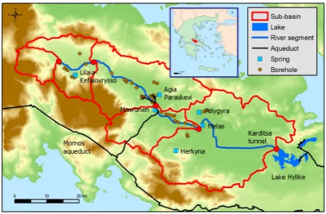
38 Figure 3: The Boeoticos Kephisos river basin and the main hydrosystem components.
Fig. 3. The Boeoticos Kephisos river basin and the main
hydrosys-tem components.
too bad against some other). Thus, the most promising part of the Pareto front is approximated, in an attempt to surround a best-compromise solution.
Regarding the evolving phase, some aspects are similar to the transitions used in the single-optimization approach, whereas some alterations are necessary to prohibit popula-tion convergence (e.g., the simplex is not allowed to shrink). Moreover, the mutation operator employs two schemes, with equal probability; one allows small perturbations around the candidate individual to die, while the other ensures the gen-eration of a random solution outside of the average range of the population.
5 Case study
5.1 The study area
The Boeoticos Kephisos river basin lies in the Eastern Sterea Hellas, north of Athens, and drains a closed area (i.e., with-out an with-outlet to the sea) of 1956 km2(Fig. 3). The catchment geology comprises heavily karstified limestone, mostly de-veloped on the mountains, and alluvial deposits, lying in the plain areas. Due to its karst subsurface, the watershed has a considerable groundwater yield. The main discharge points are large springs in the upper and middle part of the basin that account for more than half of the annual catchment runoff. Moreover, an unknown amount of groundwater is conducted to the sea.
[image:9.595.311.545.63.216.2]Table 2. Sub-basin properties.
Sub-basin 1 2 3 4 5
Area (km2) 106.2 244.8 508.8 245.9 849.9
River network length (km) – 26.0 13.0 17.2 33.3 Mean elevation (m) 957.9 707.5 520.0 470.7 286.4 Mean annual precipitation (mm) 1339.8 1001.2 922.4 974.2 698.5 Mean annual discharge∗(m3/s) 0.43 1.41 2.38 3.75 6.66
∗Computed discharge at the downstream node, comprising surface (basin) and groundwater (spring) runoff minus river abstractions.
water, significant surface and groundwater resources of the basin are used for irrigation. During the summer period, all surface water is used for irrigation, thus drying the canal at the basin outlet; in addition, part of the demand is satisfied via pumping from Hylike.
The estimation of the water balance of the basin on the basis of runoff data is impossible, because of the groundwa-ter losses, the large amounts of wagroundwa-ter infiltrating across the upper course of the river (a 25% reduction of discharge is detected, according to a series of flow measurements), and the existence of combined abstractions. Previous attempts, thought a simplified version of the model, with lumped de-scription of the main processes (Rozos et al., 2004), indi-cated that, due to the unknown distribution between evapo-transpiration and sea outflows, the problem is ill-posed, and an infinite number of solutions exist, providing similar per-formance. In the present approach, we tried to establish a much more “physical” scheme, to enhance the information content in calibration.
5.2 Model formulation and data
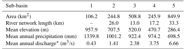
As illustrated in Fig. 3, the river network comprises a main branch, divided in four segments, and five sub-basins up-stream of or between the corresponding nodes; the main properties of the sub-basins are summarized in Table 2. For the delineation of soil processes we defined six HRUs by combining two geographical layers representing three gories of permeability (low, medium, high), and two cate-gories of terrain slope, with threshold 10% (Fig. 4; see also Table 4). These three categories of permeability were ex-tracted through aggregating detailed hydrolithological data. The low-permeable areas of the basin (21.6%) are mainly constituted by flysch, which is waterproof, the medium-permeable ones (42.8%) are generally captured by qua-ternary (alluvial) deposits, while the high-permeable areas (35.6%) are constituted by limestones of different phases, in-cluding highly karstified formations. To restrict redundant parameters, we didn’t incorporate other types of information, e.g., land use, which practically overlaps with slope, since mountainous areas are covered by forests, while plain ones are dominated by crops and, generally, low vegetation. The
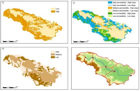
groundwater flow field is divided in 35 non-rectangular cells (Fig. 5); six of them implement surface outflows through the major karst springs, while two are located outside of the basin to simulate the draining of underground leakages to the sea. The spatial distribution of springs, with regard to the surface and groundwater system delineation, is illustrated in Figs. 3 and 5.
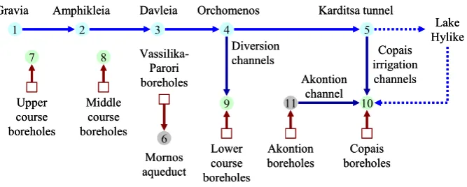
The water management network, sketched in Fig. 6, in-cludes four conceptual nodes that represent extended agri-cultural areas (totally 348 km2), six borehole groups and a dozen of aqueducts conducting abstractions from the river and the aquifer to the related nodes. Since some demands are fulfilled via multiple sources, virtual costs are assigned to the corresponding aqueducts thus representing the real manage-ment policy (i.e. priority in using surface resources, instead of the groundwater ones). Additional targets are water supply through the middle course boreholes that were drilled during the early 1990’s. Historical abstractions from Hylike are im-ported to the network as external inflows, with known values (28.9 hm3on annual average).
A. Efstratiadis et al.: HYDROGEIOS: a semi-distributed model for modified basins 999
Figure 4: Characteristic layers of geographical data for the schematization of the surface
system: (a) top left, terrain slope; (b) bottom left, permeability; (c) top right HRUs, derived as
the product of slope and permeability; (d) bottom right, river network and sub-basins.
Figure 5: Characteristic layers of geographical data for the schematization of the groundwater
system: (a) left, formulation of cells, based on permeability; (b) right, product of cells,
sub-basins, HRUs, springs and boreholes.
Fig. 4. Characteristic layers of geographical data for the schematization of the surface system: (a) top left, terrain slope; (b) bottom left,
permeability; (c) top right HRUs, derived as the product of slope and permeability; (d) bottom right, river network and sub-basins.
39
Figure 4: Characteristic layers of geographical data for the schematization of the surface
system: (a) top left, terrain slope; (b) bottom left, permeability; (c) top right HRUs, derived as
the product of slope and permeability; (d) bottom right, river network and sub-basins.
Figure 5: Characteristic layers of geographical data for the schematization of the groundwater
system: (a) left, formulation of cells, based on permeability; (b) right, product of cells,
sub-basins, HRUs, springs and boreholes.
Fig. 5. Characteristic layers of geographical data for the schematization of the groundwater system: (a) left, formulation of cells, based on
permeability; (b) right, product of cells, sub-basins, HRUs, springs and boreholes.
the allocation of runoff at the sub-basin scale, thus improv-ing the identifiability of parameters of the surface hydrologi-cal model.
With respect to groundwater level, about 20 gauges were available for the aforementioned period, mostly located in the vicinity of Boeoticos Kephisos. However, due to the differ-ence of scale between point observations and averages over the cell areas, superimposed to high heterogeneity and un-certainty of the karst aquifer, we preferred not to include this
information in calibration, i.e. we didn’t attempt any kind of “adjustment” of the simulated levels to the piezometric infor-mation. Thus, the estimation of groundwater model parame-ters was based on the observed discharge data downstream of the six springs, the empirical criteria used to avoid unrealistic trends of the simulated aquifer levels and through rough vi-sual inspection of the groundwater outputs within the hybrid calibration procedure (see next section).
[image:11.595.73.524.403.552.2]40
1 2 3 4 5
9 11 10
Gravia Amphikleia Davleia Orchomenos
7
Upper course boreholes
Copais irrigation channels Akontion
channel
Karditsa tunnel
Diversion channels 8
Middle course boreholes
Lower course boreholes
Copais boreholes Akontion
boreholes
Vassilika-Parori boreholes
Mornos aqueduct
6
Lake Hylike
Figure 6: Simplified sketch of the water management network, representing abstractions from the surface and groundwater resources. Nodes 1-5 are river points, whereas nodes 7-10 denote agricultural areas across the basin.
0.0 5.0 10.0 15.0 20.0 25.0 30.0 35.0 40.0
Oc
t-84
Oc
t-85
Oc
t-86
Oc
t-87
Oc
t-88
Oc
t-89
Oc
t-90
Oc
t-91
Oc
t-92
Oc
t-93
M
ont
hl
y di
sc
ha
rg
e
(m
3 /s
) Computed
Observed
[image:12.595.133.467.64.198.2]Figure 7: Computed and observed discharge series at the basin outlet.
Fig. 6. Simplified sketch of the water management network, representing abstractions from the surface and groundwater resources. Nodes
1–5 are river points, whereas nodes 7–10 denote agricultural areas across the basin.
The remaining hydrological inputs were monthly precipi-tation and potential evapotranspiration time series, integrated on the surface of the five sub-basins. The former were con-structed via the Thiessen method using point data from 12 rainfall stations, well-distributed through the basin, whereas the latter was estimated via the Penman-Monteith method, on the basis of land-use information. Theoretical irrigation needs were approximated by assuming an average annual value of 6500 m3/ha of irrigated land, which corresponds to an annual demand of 226 hm3with unknown (a priori) allo-cation.
5.3 Calibration strategy
The model parameters (∼100) were fitted on about 40 cri-teria, weighted in a single performance measure. These in-clude: (a) the efficiency index and the average bias, to cal-ibrate the hydrographs at the basin outlet (Karditsa tunnel) and downstream of the six karst springs; (b) the zero-flow penalty to better fitting the discharge at the outlet (systemat-ically going to zero during each irrigation period) and down-stream of the Mavroneri springs (with zero flow, in case of intensive pumping); and (c) the trend penalty to realistically represent the variability of groundwater cell levels, except for those lying in the neighbourhood of springs, the behaviour of which is better controlled though the hydrographs. The first two statistical criteria ensured satisfactory spread around the measured values and avoidance of systematic errors, while the empirical measures enhanced the information embedded in calibration (thus ensuring compatibility between model free variables and criteria involved) and helped to control much larger number of model responses than the observed ones. The 10-year control period was split in a six-year cal-ibration period (October 1984–September 1990) and a four-year validation period (October 1990–September 1994).
Given the intricacy of the derived optimization problem, it was impossible to obtain a reliable solution in a single run. Apart from the vast number of local optima and the irregular-ities of the response surface, an additional complexity factor
was the different order of magnitude between the groundwa-ter conductivities, taking values in the range 10−8to 10−1, and the rest of parameters, most of them being dimension-less. This was partly remedied using logarithms of conduc-tivities.
To deal with the multiple puzzles of the calibration prob-lem, while ensuring a satisfactory predictive capacity of the model, a hybrid calibration strategy was employed, through progressive improvements of relatively small groups of pa-rameters. At a preliminary phase, we used extended bounds for the search space and tried various combinations of weighting coefficients, to obtain a general overview of the problem, regarding the multiple criteria interactions and their feasible range.
At the second phase, we attempted to optimize the HRU parameters, as well as the most important parameters of the groundwater model, specifically the conductivities of the springs and their adjacent cells. Moreover, the interior bounds of parameters were restricted to be consistent with their broad physical interpretation. The main objective was to guarantee a good fitting of the hydrograph at the outlet, especially its parts related to high flows, and a satisfactory fitting of the spring flows. At the end of this phase, we re-moved most trend penalties, since we ensured a “regular” behaviour of the groundwater model, by appropriately ad-justing the corresponding parameters.
A. Efstratiadis et al.: HYDROGEIOS: a semi-distributed model for modified basins 1001
Table 3. Optimal values of efficiency and relative bias for the calibration and validation periods.
Monthly runoff Calibration period Validation period
Efficiency Bias∗ Efficiency Bias∗
Basin outlet 0.870 −0.054 0.756 0.107
Lilea-Kefalovrysso springs 0.806 −0.068 0.607 −0.108
Agia Paraskevi springs 0.724 −0.063 – –
Mavroneri springs 0.693 −0.106 0.601 −0.315
Herkyna springs 0.431 0.039 0.458 0.068
Melas springs 0.265 −0.008 0.095 −0.112
Polygyra springs 0.372 0.006 – –
∗
Bias = relative bias with respect to historical mean.
40
1 2 3 4 5
9 11 10
Gravia Amphikleia Davleia Orchomenos
7 Upper course boreholes Copais irrigation channels Akontion channel Karditsa tunnel Diversion channels 8 Middle course boreholes Lower course boreholes Copais boreholes Akontion boreholes Vassilika-Parori boreholes Mornos aqueduct 6 Lake Hylike
Figure 6: Simplified sketch of the water management network, representing abstractions from the surface and groundwater resources. Nodes 1-5 are river points, whereas nodes 7-10 denote agricultural areas across the basin.
0.0 5.0 10.0 15.0 20.0 25.0 30.0 35.0 40.0 Oc t-84 Oc t-85 Oc t-86 Oc t-87 Oc t-88 Oc t-89 Oc t-90 Oc t-91 Oc t-92 Oc t-93 M ont hl y di sc ha rg e (m 3/s ) Computed Observed
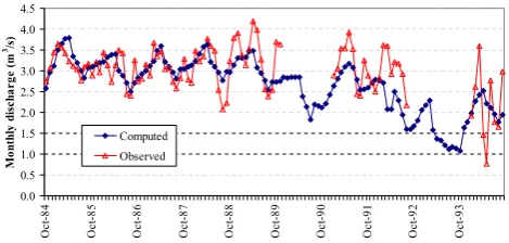
Figure 7: Computed and observed discharge series at the basin outlet. Fig. 7. Computed and observed discharge series at the basin outlet.
0.0 0.5 1.0 1.5 2.0 2.5 3.0 3.5 4.0 Oc t-84 Oc t-85 Oc t-86 Oc t-87 Oc t-88 Oc t-89 Oc t-90 Oc t-91 Oc t-92 Oc t-93 M ont hl y di sc ha rg e (m 3/s ) Computed Observed
Figure 8: Computed and observed discharge series at Lilaia-Kefalovrysso springs.
0.0 0.1 0.2 0.3 0.4 0.5 0.6 0.7 0.8 0.9 Oc t-84 Oc t-85 Oc t-86 Oc t-87 Oc t-88 Oc t-89 Oc t-90 Oc t-91 Oc t-92 Oc t-93 M ont hl y di sc ha rg e (m 3/s ) Computed Observed
Figure 9: Computed and observed discharge series at Agia Paraskevi springs.
Fig. 8. Computed and observed discharge series at Lilaia-Kefalovrysso springs.
that the model is unavoidably vulnerable to the existing mul-tiple sources of uncertainty, which is further amplified by the high complexity of the system under study.
5.4 Results and discussion
The optimized statistical measures against the simulated runoffs are summarized in Table 3, whereas Figs. 7–13 com-pare the observed and the computed hydrographs at the seven control sites. Regarding the runoff at the outlet (Fig. 7), a very good fitting is ensured for both the calibration and vali-dation periods, with efficiency values 87.0% and 75.6%,
re-41 0.0 0.5 1.0 1.5 2.0 2.5 3.0 3.5 4.0 Oc t-84 Oc t-85 Oc t-86 Oc t-87 Oc t-88 Oc t-89 Oc t-90 Oc t-91 Oc t-92 Oc t-93 M ont hl y di sc ha rg e (m 3/s ) Computed Observed
Figure 8: Computed and observed discharge series at Lilaia-Kefalovrysso springs.
0.0 0.1 0.2 0.3 0.4 0.5 0.6 0.7 0.8 0.9 Oc t-84 Oc t-85 Oc t-86 Oc t-87 Oc t-88 Oc t-89 Oc t-90 Oc t-91 Oc t-92 Oc t-93 M ont hl y di sc ha rg e (m 3/s ) Computed Observed
Figure 9: Computed and observed discharge series at Agia Paraskevi springs. Fig. 9. Computed and observed discharge series at Agia Paraskevi
springs. 0.0 0.5 1.0 1.5 2.0 2.5 3.0 3.5 4.0 Oc t-84 Oc t-85 Oc t-86 Oc t-87 Oc t-88 Oc t-89 Oc t-90 Oc t-91 Oc t-92 Oc t-93 M ont hl y di sc ha rg e (m 3/s ) Computed Observed
Figure 10: Computed and observed discharge series at Mavroneri springs.
0.0 0.2 0.4 0.6 0.8 1.0 1.2 1.4 Oc t-84 Oc t-85 Oc t-86 Oc t-87 Oc t-88 Oc t-89 Oc t-90 Oc t-91 Oc t-92 Oc t-93 M ont hl y di sc ha rg e (m 3/s ) Computed Observed
Figure 11: Computed and observed discharge series at Herkyna springs.
Fig. 10. Computed and observed discharge series at Mavroneri
springs.
spectively. The model preserves the important aspects of the hydrograph, namely the high flows and the artificial flow in-terruption during the summer due to upstream abstractions. Moreover, it reproduces the sequence of high and low flow periods, which is more prominent during the validation pe-riod. Analysis with extended historical data further validated the model capacity relating to the prediction of the basin runoff (Koutsoyiannis et al., 2007).
For the Lilaia-Kefalovrysso springs, located in the up-per course of the basin, the model provides a very satisfac-tory performance (efficiency 80.6% in calibration, 60.7% in
1002 A. Efstratiadis et al.: HYDROGEIOS: a semi-distributed model for modified basins 42 0.0 0.5 1.0 1.5 2.0 2.5 3.0 3.5 Oc t-84 Oc t-85 Oc t-86 Oc t-87 Oc t-88 Oc t-89 Oc t-90 Oc t-91 Oc t-92 Oc t-93 M ont hl y di sc ha rg e (m 3/s ) Computed Observed
Figure 10: Computed and observed discharge series at Mavroneri springs.
[image:14.595.312.544.64.176.2]0.0 0.2 0.4 0.6 0.8 1.0 1.2 1.4 Oc t-84 Oc t-85 Oc t-86 Oc t-87 Oc t-88 Oc t-89 Oc t-90 Oc t-91 Oc t-92 Oc t-93 M ont hl y di sc ha rg e (m 3/s ) Computed Observed
Figure 11: Computed and observed discharge series at Herkyna springs. Fig. 11. Computed and observed discharge series at Herkyna
springs. 43 0.0 0.5 1.0 1.5 2.0 2.5 3.0 3.5 4.0 4.5 Oc t-84 Oc t-85 Oc t-86 Oc t-87 Oc t-88 Oc t-89 Oc t-90 Oc t-91 Oc t-92 Oc t-93 M ont hl y di sc ha rg e (m 3/s ) Computed Observed
Figure 12: Computed and observed discharge series at Melas springs.
[image:14.595.51.284.64.175.2]0.0 0.2 0.4 0.6 0.8 1.0 1.2 1.4 1.6 Oc t-84 Oc t-85 Oc t-86 Oc t-87 Oc t-88 Oc t-89 Oc t-90 Oc t-91 Oc t-92 Oc t-93 M ont hl y di sc ha rg e (m 3/s ) Computed Observed
Figure 13: Computed and observed discharge series at Polygyra springs.
Fig. 12. Computed and observed discharge series at Melas springs.
validation), apart from a deviation during the winter of 1992, which was characterized by large amounts of snow in con-trast to low liquid precipitation depths.
For the Mavroneri springs, located on the middle course and very close to the water supply wells, the fitting was also very satisfactory (efficiency 69.3% in calibration, 60.1% in validation). Indeed, the model represents the two charac-teristic periods of flow intermittency, where the first (May– December 1990) is entirely due to the persistent drought of the late 1980’s, whereas the second one, lasted more than a year (end of 1992 to start of 1994), resulted as combination of unfavourable hydrological conditions and intensive use of the newly constructed boreholes. Between these extremely dry periods, an impressive increase of discharge was observed, well-represented by the model. In general, the overall fitting on this particularly important hydrograph was a major guar-antee of the model performance, especially when taking into account the high uncertainty of such a karst system.
Regarding the other springs, the model fitting was less satisfactory, although acceptable. The efficiency values achieved vary from 72.4% for the Agia Paraskevi springs (the less important of the whole system) to 26.5% for the Melas springs. The latter contribute significantly to the total basin runoff and their mechanisms are extremely complex. Previ-ous modelling attempts failed, even when detailed tools were used. For example, a simulation based on the MODFLOW achieved an efficiency value of 10% (Nalbantis et al., 2002), whereas the lumped approach of Rozos et al. (2004) attained
43 0.0 0.5 1.0 1.5 2.0 2.5 3.0 3.5 Oc t-84 Oc t-85 Oc t-86 Oc t-87 Oc t-88 Oc t-89 Oc t-90 Oc t-91 Oc t-92 Oc t-93 M ont hl y di sc ha rg e (m 3/s ) Computed Observed
Figure 12: Computed and observed discharge series at Melas springs.
0.0 0.2 0.4 0.6 0.8 1.0 1.2 1.4 1.6 Oc t-84 Oc t-85 Oc t-86 Oc t-87 Oc t-88 Oc t-89 Oc t-90 Oc t-91 Oc t-92 Oc t-93 M ont hl y di sc ha rg e (m 3/s ) Computed Observed
Figure 13: Computed and observed discharge series at Polygyra springs. Fig. 13. Computed and observed discharge series at Polygyra
springs.
a value of 19.4%, regarding the combined representation of Melas and Polygyra springs (the corresponding value for the validation period was slightly negative). Hence, the specific approach, based on a rough discretization of the groundwater field and the use of linear (i.e. Darcian) equations for describ-ing water interchanges between groundwater tanks, worked better than the generic MODFLOW, mainly regarding the preservation of the observed water balance (as indicated by the negligible bias values). Yet, the lack of extended spatial information and the uncertainties of natural mechanisms did not allow a more thorough schematization and parameteriza-tion, which would probably (but not definitely) improve the model performance.
The physical interpretation of parameters is generally dif-ficult, especially for those of the groundwater model, because of the complexity of the karst system. Table 4 shows the op-timal values of the six parameters of the soil moisture model, assigned to the corresponding HRUs. It is not surprising that the direct runoff coefficients, c, and the retention rates for percolation,µ, are mainly affected by the soil permeability, whereas the soil capacities,Smax, are more related to the ter-rain slope. Thus, the plain areas of the basin have almost twice the capacity of the mountainous ones, for the same category of permeability. On the other hand, the percola-tion rates through the high-permeable soils are significant, which explains the limited contribution of surface flows to the total water potential of the basin. Regarding the river in-filtration coefficients, their optimal values are 26.4, 8.5 and 3.1%, along the upper, middle and lower course of Boeoticos Kephisos, respectively. The significant percentage of water losses in the upstream segment is consistent with the flow measurements, as mentioned in Sect. 5.1.
[image:14.595.50.285.226.338.2]A. Efstratiadis et al.: HYDROGEIOS: a semi-distributed model for modified basins 1003
Table 4. Calibrated HRU parameters.
Slope Permeability Total area (km2) c R(mm) Smax(mm) κ λ µ
Low Low 132.2 0.054 79.1 523.2 0.351 0.036 0.046
Low High 154.1 0.006 79.1 588.8 0.564 0.031 0.235
Low Medium 679.0 0.056 79.1 443.2 0.359 0.032 0.019
High Low 288.0 0.066 85.6 227.4 0.479 0.006 0.070
High High 539.8 0.006 85.6 242.0 0.147 0.000 0.140
High Medium 158.2 0.026 85.6 263.6 0.180 0.071 0.058
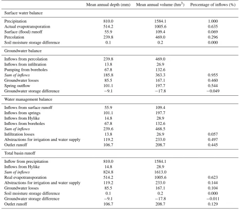
Table 5. Simulated water balance for the period 1984–1994.
Mean annual depth (mm) Mean annual volume (hm3) Percentage of inflows (%)
Surface water balance
Precipitation 810.0 1584.1 1.000
Actual evapotransporation 514.2 1005.6 0.635
Surface (flood) runoff 55.9 109.4 0.069
Percolation 239.8 469.0 0.296
Soil moisture storage difference 0.1 0.2 0.000
Groundwater balance
Inflows from percolation 239.8 469.0
Inflows from infiltration 13.8 26.9
Pumping from boreholes 67.8 132.6
Sum of inflows 185.8 363.3 0.955
Groundwater losses 85.5 167.1 0.460
Spring outflow 101.1 197.7 0.544
Groundwater storage difference −9.1 −17.8 −0.049
Water management balance
Inflows from surface runoff 55.9 109.4
Inflows from springs 101.1 197.7
Inflows from Hylike 14.8 28.9
Inflows from boreholes 67.8 132.6
Sum of inflows 239.6 468.5
Infiltration losses 13.8 26.9 0.057
Abstractions for irrigation and water supply 119.2 233.0 0.497
Outlet runoff 106.7 208.7 0.445
Total basin runoff
Inflow from precipitation 810.0 1584.1
Inflows from Hylike 14.8 28.9
Sum of inflows 824.8 1613.0
Real evapotransporation 514.2 1005.6 0.623
Abstractions for irrigation and water supply 119.2 233.0 0.144
Groundwater losses 85.5 167.1 0.104
Soil moisture storage difference 0.1 0.2 0.000
Groundwater storage difference −9.1 −17.8 −0.011
[image:15.595.50.545.244.676.2]