Goodness-of-Fit Test Based on Arbitrarily Selected Order
Statistics
Zhenmin Chen
Department of Mathematics and Statistics, FloridaInternationalUniversity, Miami, FL33199, U.S.A. *Corresponding Author: [email protected]
Copyright © 2014 Horizon Research Publishing All rights reserved.
Abstract
Checking whether or not the population distribution, from which a random sample is drawn, is a specified distribution is a popular topic in statistical analysis. Such a problem is usually named as goodness-of-fit test. Numerous research papers have been published in this area. The purpose of this short paper is to provide a goodness-of-fit test statistic which works for many kinds of censored data formed by order statistics. This is an extension of the work presented in Chen and Ye (2009). The method can be used for censoredsamplesthat are commonly used in reliability analysis including left censored data, right censored data and doubly censored data.Keywords
Goodness-of-Fit Test, Censored Data, Arbitrarily Selected Order Statistics, Uniformity1. Introduction
The goodness-of-fit test has its long history. The primary goal of the goodness-of-fit test is to check how well a specificstatistical model can fit a given data set. The
χ
2 test (Pearson (1900)), Kolmogorov-Smirnov test (Kolmogorov (1933) and Smirnov (1939)), Cramer-von Mises test (Cramer (1928)),and Anderson-Darling test (Anderson and Darling (1952)) are the statistical testspresented in early papers and are still widely used by statistics practitioners. All these test statistics are adopted by most statistical software. The Shapiro and Wilk test (Shapiro and Wilk (1965)) is another commonly used test statistic which works specifically for the normal distribution and lognormal distribution. In the recent years, many research papers have been published in the area of goodness-of-fit test. The power of the goodness-of-fit tests has been compared by many authors. See, for examples, Choulakian, Lockhart and Stephens (1994), and Steele and Chaseling (2006). Chen and Ye (2009) proposed a test statistic for checking whether or not the population distribution, from which a random sample is drawn, is a uniform distribution. It has been shown in that paper that the power of the proposed test in that paper is higher than some of the existing test statistics in some cases,especially for the case that the alternative distributions are V-shaped distributions. In this short paper, the method used in Chen and Ye (2009) will be extended to censored samples. The new test statistic can be used when only some order statistics are available.
2. Uniformity Test Based on Order
Statistics
The purpose of the uniformity test is to check whether or not the population distribution, from which a random sample was drawn, is a uniform distribution on interval
[ ]
0.1 . Suppose X X1, 2, , Xn form a random sample from apopulation distribution with support set
[ ]
0,1. Suppose also thatX X
( )1,
( )2, ,
X
( )n are the corresponding order statistics. For the complete sample case, atest statistic was proposed in Chen and Ye (2009). The test statistic has the form(
)
(
)
2 1
( ) ( 1) 1
1 2
1 1
1 , , ,
n
i i i
n
n X X
n
G X X X
n
+
− =
+ − −
+
=
∑
. (1)
Here X( )0 is defined as 0, and X(n+1) is defined as 1. Chen and Ye (2009) discussed the properties of this test statistic. The expected value, variance and the shape of this test statistic are described in that paper. When the population distribution is the same as the specified distribution, the value of G X X
(
1, , ,2 Xn)
should be pretty close to 0. On the other hand, when the population distribution is far away from the specified distribution, the value of(
1, , ,2 n)
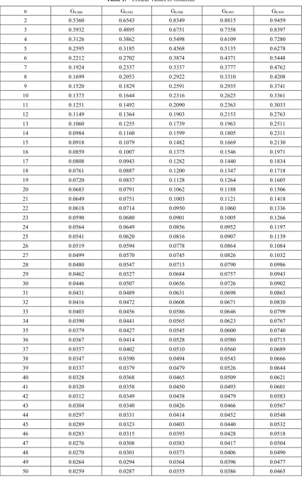
G X X X should be pretty close to 1. The quantiles of the test statistics were obtained by Monte Carlo simulation and were tabulated. In order to let statistics users find the quantile values easily, the quantile value for different sample sizes and different significance levels are listed in Table 1. The quantiles can be used to conduct goodness-of-fit test discussed in this paper. In fact, the hypothesis of uniformity should be rejected at significant level α if
(
1, , ,2 n)
1 .Table 1. Critical Values of Gstatistic
n G0.900 G0.950 G0.990 G0.995 G0.999
This paper focuses on the case that the samples are incomplete. In practice, the available samples may be censored ones. For example, in reliability analysis, the statistical analysis is usually based on left censored samples, right censored samples, or doubly censored samples. To fit the need of such kind of applications and even more generalized situations, it is assumed in this paper that only some of the order statistics are available for testing the hypotheses mentioned above. More specifically, it is assumed that only k order statistics
( )i1 ( )i2 ( )ik
X
≤
X
≤
≤
X
are available when the test is conducted. Here
1
≤ < <
i i
1 2
< ≤
i
kn
are k integers that are arbitrarily picked from set{
1,2, ,
n
}
. In such a case, the test statistic can be defined as( ) ( ) ( )
(
)
( )(
)
(
)
( ) ( )1 2 1
2 2 1 1 1 2 1 2 1 1 1 , , , 1 1
k j j
k
j j
i i i k i i
j j j j
i i n
G X X X X X
n i i n − + − + = − = − + = − − + − + −
∑
∑
(2)
for any
1
≤ < <
i i
1 2
< ≤
i
kn
. Herei
0 is defined as 0,i
k+1 is defined asn
+
1
, The test statistic defined in (2) possesses some properties. It can be seen that 0≤G X(
( )i1 ,X( )i2 , , X( )ik)
≤1. This is because( ) ( )1
(
)
(
)
2
1 1 2
1 1 2 1 1
1
1
0
.
1
1
1
j j k k j j j j i i j ji i
n
i i
X
X
n
n
n
− + + − − = =−
−
−
≤
−
−
≤
+
+
+
+
∑
∑
To show ( ) ( )
(
)
(
)
1
2
1 1 2
1
1 2
1 1
1 1 ,
1 1 1 j j k k j j j j i i j j
i i n i i
X X n
n n − + + − − = = − − ≤ + − − − + + +
∑
∑
note that( ) ( )1
2 1
1
1 j j
1
k j j i i j
i i
X
X
n
− + − =−
−
−
+
∑
( ) ( )(
1)
(
( ) ( )1)
2
1 2 1 1
1 1
1 1 1
=
2
1
1
j j j j
k k k
j j j j
i i i i
j j j
i i
i i
X
X
X
X
n
n
− − + + + − − = = =−
−
−
+
−
−
+
+
∑
∑
∑
( ) ( )(
1)
(
)
(
)
(
( ) ( )1)
1 2 1 2 1 2
1 2
1 1 1
1
2
1
1
j j j j
k k k
i i j j i i
j j j
X
X
i i
X
X
n
n
− − + + + − = = =−
−
−
≤
+
−
+
+
∑
∑
∑
( ) ( )(
1)
(
)
(
)
1 2 1 2
1 2
1 1
1
1
1
j j1
k k
i i j j
j j
n
X
X
i i
n
−n
+ + − = =
−
−
−
=
+
+
∑
+
∑
( ) ( )(
1)
(
)
(
)
(
)
(
)
2
1 1 2 1 2
1 1
2 2
1 1 1
1
1
1
1
.
1
j j1
1
1
k k k
i i j j j j
j j j
n
X
X
i i
n
i i
n
−n
n
n
+ + + − − = = =
−
−
−
−
−
≤
+
≤
+
+
∑
+
∑
+
+
∑
It can also be seen that
(
( )i ( 1)i)
1
1
E X
X
n
−
−
=
+
for any
i
=
1,2, ,
n
+
1.
It implies that(
1)
1(
)
( )j (j )
1
1,2, ,
1
.
j j
i i
i i
E X
X
j
k
n
− −−
−
=
=
+
+
Therefore, the value of
G X
(
( )i1,
X
( )i2, ,
X
( )ik)
should be quite close to zero if the population distribution is the uniformThen H0 should be rejected at significant level
α
if( ) ( ) ( )
(
i1 , i2 , , ik)
1(
1 2, , , k)
G X X X >G−α i i i
. Here
G
1−α(
i i
1 2, , ,
i
k)
is a number such that( ) ( ) ( )
(
)
(
)
(
i1 , i2 , , ik 1 1 2, , ,k)
P G X X X >G−α i i i =
α
.
For the complete sample case, the critical values computed in Chen and Ye (2009) can be adopted to conduct the statistical test discussed in this section. For such a general case, a simple computer program is needed to run Monte Carlo simulation to find the critical values of the test statistic.
3. Test for General Distributions
Now suppose
X X
1,
2, ,
X
nform a random sample from a population distribution with cumulative distribution function( )
0
F x
. Suppose also thatX X
( )1,
( )2, ,
X
( )n are the corresponding order statistics. The purpose is to test0
H
: The cumulative distribution function of the population distribution isF x
0( )
,a
H
: The cumulative distribution function of the population distribution is notF x
0( )
. It is well known that0
( ), ( ),...., ( )
1 0 2 0 nF X F X
F X
form a random sample from the
U
[ ]
0,1
distribution. Then( ) ( ) ( )
0
(
1), (
0 2),...., (
0 n)
F X
F X
F X
are the ordered observations of a random sample from the
U
[ ]
0,1
distribution because of the monotonic property of the cumulative distribution function. Therefore, testing whether or not the cumulative distribution of the population, from which1
,
2, ,
nX X
X
are sampled, isF x
0( )
is the same as testing whether or not the population distribution, from which0
( ), ( ),...., ( )
1 0 2 0 nF X F X
F X
are sampled, is the uniform distribution on[ ]
0,1
. For the complete sample case, the test statistic can be defined as(
)
(
)
2 1
0 ( ) 0 ( 1) 1
1 2
1
1 ( ) ( )
1 , , ,
n
i i
i n
n F X F X
n
G X X X
n
+
− =
+ − −
+
=
∑
(3)
Here
X
( )0 is defined as−∞
0, andX
(n+1) is defined as+∞
.The hypothesis In fact,H
0should be rejected at significant level α ifG X X
(
1, , ,
2
X
n)
>
G
1−α.
Now it is assumed that only k order statistics
( )i1 ( )i2 ( )ik
X
≤
X
≤
≤
X
are available when the test is conducted. Here
1
≤ < <
i i
1 2
< ≤
i
kn
are k integers that are arbitrarily picked from set{
1,2, ,
n
}
. Then the test statistic can be defined as( ) ( ) ( )
(
)
(
)
(
)
(
)
( )
( )(
( )1)
1 2
2
2 1
1
1 2 0 0
1 2
1 1
1 , , ,
1
1 j j
k
k
j j
i i
i i i k
j j j j
i i
n X X
G X X X F F
n i i
n −
+
− +
= − =
−
+
= − − +
− +
−
∑
∑
(4)
as
−∞
andX
( )ik+1 is defined as+∞
. The null hypothesisH
0should be rejected at significance levelα
if( ) ( ) ( )
(
i1,
i2, ,
ik)
1(
1 2, , ,
k)
G X
X
X
>
G
−αi i
i
.The value of
G
1−α(
i i
1 2, , ,
i
k)
can be obtained using Monte Carlo simulation for any combination ofi i
1 2, , ,
i
kandα
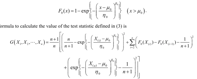
.For example, suppose the test mentioned above is used to check if the population distribution of a data set is a three-parameter Weibull distribution with location parameter
µ
0, shape parameterβ
0 and scale parameterη
0. The cumulative distribution function of the three-parameter Weibull distribution is(
)
0
0
0 0
0
( ) 1 exp
x
F x
x
β
µ
µ
η
−
= −
−
>
.Then the formula to calculate the value of the test statistic defined in (3) is
(
)
( )0 2 2
0 1
1 2 0 ( ) 0 ( 1)
2 0
1 1
, , , exp ( ) ( )
1 1
n
n i i
i
X
n n
G X X X F X F X
n n n
β
µ
η −
=
−
+
= − − + − −
+ +
∑
( )
0 2
0
0
1
exp
1
nX
n
β
µ
η
−
+
−
−
+
for complete samples. The calculated value of
G X X
(
1, , ,
2
X
n)
can then compared with the critical value listed inTable 1 to determine whether or not to reject the null hypothesis that the population distribution is the three-parameter Weibull distribution.
For the samples containing k order statistics only, the formula to calculate the value of the test statistic defined in (4) becomes
( ) ( ) ( )
(
)
(
)
(
)
(
)
( )1 0
1 2
2 2
0 1
1 2
2 1 0
1
1
1
,
, ,
exp
1
1
k
i
i i i k
j j j
X
n
i
n
G X
X
X
n
i i
n
β
µ
η
+− =
+ −
−
+
=
−
−
+
−
+
−
∑
( )
( )
(
( ))
( )0
1
2 2
0 1
0 0
1 0
1
exp
1
1
k
j j
k
i
j j k
i i
j
X
i i
n
i
X
X
F
F
n
n
β
µ
η
−
− =
−
−
+ −
+
−
−
+
+
−
−
+
∑
.
[image:5.595.98.497.208.369.2]4. Conclusion and Discussion
In this short paper, a goodness-of-fit test statistic is proposed for checking whether or not the cumulative distribution function of a population distribution has a specified form for the case that sampled data are arbitrarily censored. More specifically, the test is performed based on order statistics
X
( )i1≤
X
( )i2≤
≤
X
( )ik for arbitrarily selected1
≤ < <
i i
1 2
< ≤
i
kn
. Such a setting covers various censoring cases used in reliability analysis and other fields. Because of its flexibility in regard of selection of sample items, the method can be used for many complicated cases. For example, in life test, the data collectors may collect failure times during one time period and leave the test items running without observing the failure times in the second time period. Then the data collectors may come back and record failure times in the third time period. The procedure can continue with the same pattern. The method presented in this paper can be used for this kind of data without any technical difficulties. It has been shown that the value of the proposed test statistic is always between 0 and 1. The critical values of the proposed test statistic can be obtained by Monte Carlo simulation. The test statistic discussed in Chen and Ye (2009) is for univariate uniformity. By applying the probability integral transformation, the test can be used to check if the cumulative distribution of a population distribution is of any specified distribution. It is worth being noted here is that the test statistic discussed in this paper is for testing whether or not the population distribution, from which a random sample is drawn, is a specified distribution. It means that everything about the distribution is known. In practice, however, sometimes it is desired to test if the population distribution is of certain type when the parameters of the distribution are unknown. In that case, it is believed that the method suggested by Lilliefors (Lilliefors (1967) and Lilliefors (1969)) can be used.REFERENCES
[1] Anderson, T. W. and Darling, D. A. (1952) Asymptotic Theory of Certain “Goodness of Fit” Criteria Based on Stochastic Process, Annals of Mathematical Statistics, 23, 193-212.
[2] Chen, Zhenmin and Ye, Chunmiao (2009) An alternative test for uniformity, International Journal of Reliability, Quality and Safety Engineering, 16, 343-356.
[3] Choulakian, V., Lockhart, R. A. and Stephens, M. A. (1994) Cramer-von Mises Statistics for Discrete Distributions, The Canadian Journal of Statistics, 22, 125-137.
[4] Cramer, H. (1928) On the Composition of Elementary Errors, SkandinaviskAktuarietidskrift, 11,13-74, 141-180.
[5] Kolmogorov, A. N. (1933) Sulla Determinazione Empirica di Una Legge di Distribuzione, Giornale dell’ Istituto degli Attuari, 4, 83-91.
[6] Lilliefors, W. H. (1967) On the Kolmogorov-Smirnov test for normality with mean and variance unknown, Journal of the American Statistics Association, 62, 399-402.
[7] Lilliefors, W. H. (1969) On the Kolmogorov-Smirnov test for the exponential distribution with mean unknown, Journal of the American Statistics Association, 64, 387-389.
[8] Pearson, K. (1900) On the Criterion that a Given System of Deviations from the Probable in the Case of a Correlated System of Variables is such that it can be Reasonably Supposed to Have Arisen from Random Sampling, Philosophical Magazine, 5, 157–175.
[9] Shapiro, S. S. and Wilk, M. B. (1965) An analysis of variance test for normality (complete samples), Biometrika, 52, 591-611.
[10] Smirnov, N. V. (1939) Estimate of Deviation Between Empirical Distributions (Russian), Bulletin Moscow University, 2, 3-16.