Numerical Schemes and Monte Carlo Method for Black and Scholes Partial Differential Equation: A Comparative Note

(1)

Numerical Schemes and Monte Carlo Method for

Black and Scholes Partial Differential Equation: A

Comparative Note

Sharif Mozumder

*

_{, ABM Shahadat Hossain, Sadia Tasnim, Arafatur Rahman}

Department of Mathematics, University of Dhaka, Bangladesh

Abstract

This paper comparatively investigates some iterative methods and Monte Carlo simulation technique for the dynamics underlying the celebrated Black and Scholes (BS) model. In particular we attempt to answer the question: ‘How many Monte Carlo replications can yield prices, for plain vanilla type European derivatives on a stock, which are similar to those obtained by solving the BS PDE using iterative numerical schemes?’ We confine to three frequently referred iterative schemes such as Successive over Relaxation (SOR), Gauss-Seidel (GS) and Jacobi (JC). This information together with the information of ‘differences in time requirements’ will help to guess the similar trade-offs for complex derivatives(exotic) pricing for which there are no analytic pricing formulas.

Keywords

Black and Scholes PDE, Iterative Solutions, Monte Carlo Simulation, Option Pricing

1. Introduction

Modern option pricing techniques are often considered among the most mathematically complex area among all applied areas of finance. A vanilla option (normal call or put option) is a financial instrument that gives the holder the right, but not the obligation, to buy or sell an underlying asset at a predetermined price, within a given time frame and it is generally traded on an exchange such as the Chicago Board Options Exchange. In this paper we deal with two approaches in derivative pricing under Black and Schole’s world. One approach is preferred by people in computational mathematics area and another approach falls under the concern of people from stochastic finance area. The first approach concerns iterative methods to solve the Black-Scholes (BS) type partial differential equation in order to price different financial products traded on some underlying, which is often an index or individual stock. The second approach concerns the so called Monte Carlo (MC)

simulation to pricing various financial products. This approach replicates random phenomena which are hypothesized to capture the reality. While the numerical methods are algorithmic and can be applied to most of the PDE’s, the Monte Carlo methods are time consuming and depends upon the number of replications considered in order to price some particular financial product under consideration. We shed some light on the trade-offs between the approaches for basic vanilla type derivative pricing.

We revisit different iterative methods used in numerically solving BS PDE in order to obtain the fair price of the vanilla options. We consider Jacobi (JC), Gauss-Seidel (GS) and Successive-Over-Relaxation (SOR) algorithms with backward substitution to price plain vanilla put options. The iterative methods are studied in great details by Burden[3], Isaacson[7], Atkinson [1] ; and their stochastic versions are explored by Mao [9], Kloeden [10].

(2)

always better than those obtained by iterative schemes. Comparisons for illustrative options are presented through tables showing the trade-offs between the approaches.

The paper is structured as follows: section 2 briefly revisits the BS PDE and BS pricing. Section 3 is about the option pricing under MC simulation. We briefly discuss the iterative methods under consideration in section 4. Section 5 shows how one can price options using the iterative methods. We conduct numerical implementation and discuss our findings in section 6. Section 7 concludes the paper.

2. BS PDE

The Black–Scholes equation is a partial differential equation which describes the evolution of an option price over time. The key idea behind the equation is that one can perfectly hedge the option by buying and selling the underlying asset and consequently “eliminate risk". This hedge, in turn, implies that there is only one right price for the option, as returned by the Black–Scholes formula. We consider the BS PDE formula for analytic pricing as we will compare the analytic prices both with numerical prices(coming from solving the BS PDE using iterative methods) as well as prices obtained by applying MC simulation to BS dynamics.

For European style option with pay-off ‘V’ the celebrated BS equation is (see Black and Schole[2]) :

𝛿𝛿𝛿𝛿 𝛿𝛿𝛿𝛿 +

1 2𝜎𝜎2𝑆𝑆2 𝛿𝛿

2_𝛿𝛿

𝛿𝛿𝑆𝑆2+rS 𝛿𝛿𝛿𝛿_{𝛿𝛿𝑆𝑆}− 𝑟𝑟𝑟𝑟 = 0.

The values of call option, 𝐶𝐶(𝑆𝑆, 𝑡𝑡) and put option 𝑃𝑃(𝑆𝑆, 𝑡𝑡)

for a non-dividend paying underlying stock in terms of the Black–Scholes paradigm are:

𝐶𝐶(𝑆𝑆, 𝑡𝑡) = 𝑁𝑁(𝑑𝑑1)𝑆𝑆 − 𝑁𝑁(𝑑𝑑2)𝐾𝐾𝑒𝑒−𝑟𝑟(𝑇𝑇−𝛿𝛿) , 𝑓𝑓𝑓𝑓𝑟𝑟𝐶𝐶𝑓𝑓𝑓𝑓𝑓𝑓𝑓𝑓𝑓𝑓𝑡𝑡𝑓𝑓𝑓𝑓𝑓𝑓

𝑃𝑃(𝑆𝑆, 𝑡𝑡) = 𝑁𝑁(−𝑑𝑑2)𝐾𝐾𝑒𝑒−𝑟𝑟(𝑇𝑇−𝛿𝛿)− 𝑁𝑁(−𝑑𝑑1)𝑆𝑆 , 𝑓𝑓𝑓𝑓𝑟𝑟𝑃𝑃𝑓𝑓𝑡𝑡𝑓𝑓𝑓𝑓𝑡𝑡𝑓𝑓𝑓𝑓𝑓𝑓�

(1) Here the price put option is based on put-call parity. In(1):

𝑑𝑑1=

𝑙𝑙𝑙𝑙�_𝐾𝐾𝑆𝑆�+�𝑟𝑟+𝜎𝜎2₂�(𝑇𝑇−𝛿𝛿) 𝜎𝜎√𝑇𝑇−𝛿𝛿

𝑑𝑑2=

𝑙𝑙𝑙𝑙�_𝐾𝐾𝑆𝑆�+�𝑟𝑟−𝜎𝜎2₂�(𝑇𝑇−𝛿𝛿) 𝜎𝜎√𝑇𝑇−𝛿𝛿

= 𝑑𝑑1− 𝜎𝜎√𝑇𝑇 − 𝑡𝑡

⎭ ⎪ ⎪ ⎬ ⎪ ⎪ ⎫

(2)

For both the option pricing formulas as in (1), 𝑁𝑁(. )is the cumulative distribution function of the standard normal distribution, (𝑇𝑇 − 𝑡𝑡) is the time to maturity, 𝑆𝑆is the stock price of the underlying asset, 𝐾𝐾 is the strike price, 𝜎𝜎 is the volatility of returns of the underlying asset and ‘r’ is the annual risk free rate.

3. Option Pricing Using Monte Carlo

Simulation

Monte Carlo Simulation is used in finance to value and analyze instruments, portfolios and investments by simulating the various sources of uncertainty which affect their values, and then determining their average values over the range of resultant outcomes. This is usually done by stochastically simulating the price patterns of the underlying on which the derivatives are traded. For option pricing, the technique involved the following operations, see Hull [6], Higham [5], Jackel[8]:

(1) To generate several thousand possible (but random) price paths for the underlying via simulation.

(2) To calculate the associated exercise value (i.e. "payoff") of the option for each path.

(3) To average these pay offs. This result is the value of the option.

(4) To discount this value to the present value.

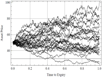
Usually a large number of asset path are generated that evolve according to the equation:

𝑑𝑑𝑆𝑆 = 𝜎𝜎𝑆𝑆𝑑𝑑𝜎𝜎 + 𝑟𝑟𝑆𝑆𝑑𝑑𝑡𝑡 (3)

(3)

[image:3.595.135.477.74.329.2]

Figure 1. Multiple Monte Carlo generated price paths

4. Iterative Methods

An iterative method is a mathematical procedure that generates a sequence of improved approximation to the solutions for a class of problems. In the process of finding a solution of a system of equations, an iterative method uses an initial guess to generate successive approximations to a solution. We show application of three frequently referred iterative techniques namely: Jacobi (JC), Gauss-Seidel (GS) and Successive-Over-Relaxation (SOR) which produce the numerical solutions for BS PDE. In general we solve a system 𝑥𝑥 = 𝑏𝑏 ; 𝐴𝐴 being a matrix and 𝑥𝑥 and 𝑏𝑏 are column vectors. See Atkinson [1], Isaacson[7].

Jacobi (JC) method is the simplest of all three iterative methods we consider. It uses the 𝑘𝑘𝛿𝛿ℎ_{value of the} approximation to determine the (𝑘𝑘 + 1)𝛿𝛿ℎ_{approximation.} The GS(or the method of successive displacement) is an iterative method, used to solve a linear system of equations, which is simple modification of the Jacobi method. Though it can be applied to any matrix with non-zero elements on the diagonals, convergence is only guaranteed if the matrix is either diagonally dominant or symmetric and positive definite. GS iterative method uses the recent approximations, instead of 𝑘𝑘𝛿𝛿ℎ_{value, to determine the}_{(𝑘𝑘 + 1)}𝛿𝛿ℎ_{value. See} Atkinson (1978), Isaacson (1994). The last iterative method of our consideration SOR is a variant of the GS method for solving a linear system of equations. SOR iterative method is the modification of GS iterative method. SOR iterative method uses the (𝑘𝑘 + 1)𝛿𝛿ℎ _{approximation with a} relaxation parameter 𝜔𝜔 as a modification of GS method. Among the three iterative methods SOR gives faster result, as it converges faster than other two iterative methods. An algorithmic view of three iterative methods looks like as below:

𝑓𝑓𝑓𝑓𝑟𝑟 𝑘𝑘 = 1,2, . . . n 𝑑𝑑𝑓𝑓

𝑓𝑓𝑓𝑓𝑟𝑟 𝑓𝑓 = 1,2, . . . , 𝑓𝑓 𝑑𝑑𝑓𝑓

Jacobi method:

𝑧𝑧𝑖𝑖𝑘𝑘+1=_𝑓𝑓1

𝑖𝑖𝑖𝑖�𝑏𝑏𝑖𝑖− � 𝑓𝑓𝑖𝑖𝑖𝑖𝑥𝑥𝑖𝑖 𝑘𝑘 𝑖𝑖−1

𝑖𝑖=1 − � 𝑓𝑓𝑖𝑖𝑖𝑖𝑥𝑥𝑖𝑖

𝑘𝑘 𝑙𝑙

𝑖𝑖=𝑖𝑖+1 �

𝑥𝑥𝑖𝑖𝑘𝑘+1 = 𝑥𝑥𝑖𝑖𝑘𝑘+ 𝑧𝑧𝑖𝑖𝑘𝑘+1

Gauss-Seidel method:

𝑧𝑧𝑖𝑖𝑘𝑘+1 =_𝑓𝑓1

𝑖𝑖𝑖𝑖�𝑏𝑏𝑖𝑖− � 𝑓𝑓𝑖𝑖𝑖𝑖𝑥𝑥𝑖𝑖 𝑘𝑘+1 𝑖𝑖−1

𝑘𝑘 𝑙𝑙

𝑥𝑥𝑖𝑖𝑘𝑘+1 = 𝑥𝑥𝑖𝑖𝑘𝑘+ 𝑧𝑧𝑖𝑖𝑘𝑘+1

SOR method:

𝑧𝑧𝑖𝑖𝑘𝑘+1 =_𝑓𝑓1

𝑖𝑖𝑖𝑖�𝑏𝑏𝑖𝑖− � 𝑓𝑓𝑖𝑖𝑖𝑖𝑥𝑥𝑖𝑖 𝑘𝑘+1 𝑖𝑖−1

𝑘𝑘 𝑙𝑙

𝑥𝑥𝑖𝑖𝑘𝑘+1= 𝜔𝜔𝑧𝑧𝑖𝑖𝑘𝑘+1+ (1 − 𝜔𝜔) 𝑥𝑥𝑖𝑖𝑘𝑘

end i; end k;

5. Pricing Options Using Iterative

Methods

We use an implicit Euler characterization of finite difference method for our illustration. For our bivariate, parabolic PDE, we start by establishing a rectangular solution domain in the two variables, 𝑆𝑆&𝑡𝑡; and then apply finite difference approximations to each of the derivative terms in the PDE. Consider the domain discretisation in𝑆𝑆&𝑡𝑡: Asset Value

(4)

Time Discretisation:{0, 𝛿𝛿t, 2𝛿𝛿t, 3𝛿𝛿t, . . . , 𝑀𝑀𝛿𝛿𝑡𝑡}where𝑁𝑁𝛿𝛿𝑡𝑡 = 𝑇𝑇

and 𝑟𝑟𝑖𝑖,𝑖𝑖= 𝑟𝑟(𝑓𝑓𝛿𝛿𝑆𝑆, 𝑗𝑗𝛿𝛿𝑡𝑡) 𝑓𝑓 = 0,1, … , 𝑀𝑀 𝑗𝑗 = 0,1, … , 𝑁𝑁

𝑆𝑆𝑚𝑚𝑚𝑚𝑚𝑚 is a maximum value for 𝑆𝑆that we must choose sufficiently large (of course, a discretization cannot allow S to assume infinity!). Following boundary conditions are for European Put options:

V (𝑆𝑆, 𝑑𝑑𝑇𝑇) = max�𝐾𝐾– 𝑆𝑆, 0�V (0, t) = 𝐾𝐾e−r(T−t)_{V (𝑆𝑆}

𝑚𝑚𝑚𝑚𝑚𝑚, t) = 0 … … … (4) In mesh-grid notations:

𝑟𝑟𝑖𝑖,𝑁𝑁 = max(𝐾𝐾 − (𝑓𝑓𝛿𝛿𝑆𝑆), 0) 𝑓𝑓 = 0,1, … , 𝑀𝑀

𝑟𝑟0,𝑖𝑖 = 𝐾𝐾𝑒𝑒−𝑟𝑟(𝑁𝑁−𝑖𝑖)𝛿𝛿𝛿𝛿𝑗𝑗 = 0,1, … , 𝑁𝑁

𝑟𝑟𝑀𝑀,𝑖𝑖= 0 𝑗𝑗 = 0,1, … , 𝑁𝑁

For a given payoff at expiry, our problem is to solve the Black-Scholes PDE backwards in time from expiry to the present time (t = 0). If all three derivative terms are approximated with Implicit Euler finite difference the discretisation is given by:

( )

2

, , 1 1, 1 , 1 1, 1

2

1, 1 1, 1

, 1 2

2

1

2

0

i j i j i j i j i j

i j i j

i j

V

i S

t

S

V

r i S

rV

S

δ

− + − − − −

+ − − −

−

+

−

+

−

=

(5)

This uses a backward difference to approximate the time derivative (since we are solving backward in time from expiry) and a central difference to approximate the first derivative in asset value. The second derivative term is approximated by the usual second difference.

Upon simplification, we can re-write (5) as:

𝑟𝑟𝑖𝑖,𝑖𝑖 = 𝐴𝐴𝑖𝑖𝑟𝑟𝑖𝑖−1,𝑖𝑖−1+ 𝐵𝐵𝑖𝑖𝑟𝑟𝑖𝑖,𝑖𝑖−1+ 𝐶𝐶𝑖𝑖𝑟𝑟𝑖𝑖+1,𝑖𝑖−1; where

𝐴𝐴𝑖𝑖=1_{2 𝛿𝛿𝑡𝑡}(𝑟𝑟𝑓𝑓 − 𝜎𝜎2𝑓𝑓2); 𝐵𝐵𝑖𝑖= 1 + (𝜎𝜎2𝑓𝑓2+ 𝑟𝑟)𝛿𝛿𝑡𝑡; 𝐶𝐶𝑖𝑖

= − 1₂𝛿𝛿𝑡𝑡(𝑟𝑟𝑓𝑓 + 𝜎𝜎2_𝑓𝑓2₎

We can now apply iterative methods using these formulas to price options.

6. Numerical Implementation

We produce the results for put options and one can have the similar analysis for call options using put-call parity. We replicate various numbers of paths to price each option and found that MC method is more powerful than numerical schemes even with relatively less number of replication to price each option. We compare the Monte Carlo simulation with the three iterative methods using the illustrative parameter values as value of the underlying, S = 5, the volatility 𝜎𝜎 =0.31_{, risk free interest rate r = .06, time to}

expiry T=1,n umber of time and asset mesh points N=500. Of course in particular context these parameter sets could be quite different and some parameters might have some effect on numerical schemes and/or MC method as well. However we ignored that issue in this research. We compare each of the numerical schemes with different number of replications in MC pricing. We then choose 24_{and 2}10_{replications to}

draw the graphs showing the comparison of iterative methods with MC method. Figure 2 shows the trade-offs between number of replications and corresponding price differences for each of the numerical schemes and MC method.

Table1. Price comparison of Monte Carlo simulation and iterative numerical methods.

No of Monte Carlo Paths

Prices

Jacobi Gauss Seidel SOR Monte _Carlo

24

0.4526 0.4663 0.4723 0.7620

210 _0.4514

Table2.Time comparison of Monte Carlo simulation and iterative numerical methods.

No of Monte Carlo Paths

Elapsed Time(sec) for prices

Jacobi Gauss Seidel SOR Monte _Carlo

24

16.4629 13.3019 12.1938 3.1839

210 143.28

97

From the results in table 1 we can say that there is hardly any difference in SOR, GS & JC iterative methods for European option pricing. We get little bit better prices for SOR method compared to GS and JC methods; however the difference is really negligible. Nonetheless little preference can go with SOR among the numerical methods. Our main concern is how many paths can ensure that MC prices are in the close proximity of numerical prices. We found that for number of paths gradually increasing from 24_{to 2}10_{the MC}

prices become gradually closer to numerical prices. It is not impossible to get MC prices with as little as 24_replications

which are well comparable with the prices obtained by with any of the numerical schemes. However, more importantly we observe that for number of replications being near 210_it

is almost always the case that

1_{For very small}_𝜎𝜎_{values there is concern on obtaining the convergence in} numerical schemes; see e.g. [12], [13].

(5)

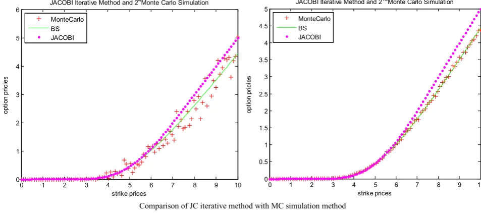
Comparison of JC iterative method with MC simulation method

Comparison of GS iterative method with MS simulation method

[image:5.595.64.541.83.294.2]

Comparison of SOR iterative method with MC simulation method

Figure 2. Comparison of iterative and MC methods.

0 1 2 3 4 5 6 7 8 9 10

0 1 2 3 4 5 6

strikeprices

opt

ion

pr

ic

ies

JACOBI Iterative Method and 24Monte Carlo Simulation MonteCarlo

BS JACOBI

0 1 2 3 4 5 6 7 8 9 10

0 0.5 1 1.5 2 2.5 3 3.5 4 4.5 5

strikeprices

opt

ion

pr

ic

ies

JACOBI Iterative Method and 210Monte Carlo Simulation MonteCarlo

BS JACOBI

0 1 2 3 4 5 6 7 8 9 10

0 0.5 1 1.5 2 2.5 3 3.5 4 4.5 5

strikeprices

opt

ion

pr

ic

ies

GS Iterative Method and 24Monte Carlo Simulation MonteCarlo

BS GS

0 1 2 3 4 5 6 7 8 9 10

0 0.5 1 1.5 2 2.5 3 3.5 4 4.5 5

strikeprices

opt

ion

pr

ic

ies

GS Iterative Method and 210Monte Carlo Simulation MonteCarlo

BS GS

0 1 2 3 4 5 6 7 8 9 10

0 0.5 1 1.5 2 2.5 3 3.5 4 4.5 5

strikeprices

opt

ion

pr

ic

ies

SOR Iterative Method and 24Monte Carlo Simulation MonteCarlo

BS SOR

0 1 2 3 4 5 6 7 8 9 10

0 0.5 1 1.5 2 2.5 3 3.5 4 4.5 5

strikeprices

opt

ion

pr

ic

ies

SOR Iterative Method and 210Monte Carlo Simulation MonteCarlo

(6)

MC prices are in very close proximity to the prices coming from any of the numerical schemes. Furthermore comparing with analytic BS prices it is clear that with more number of replications in MC prices can be made increasingly closer to those obtained with analytic BS formula, however only at the expense of additional computational time. With respect to equally comparable pricing, however, numerical iterative prices are much faster than MC prices; as is evident from table 1 and table 2. Though only reported for an illustrative option type these observations are found true for other maturity options as well as other types (e.g. European Call).

7. Conclusions

In this paper we studied iterative methods and the Monte Carlo simulation method for the dynamics underlying the celebrated Black and Scholes (BS) model in order to see the trade-offs between the approaches. We tried various numbers of replications under MC method in order to see how simulation based pricing fares with iterative pricing. Our observation is that if one is comfortable with little bit more time requirementi_{then MC prices are much better than}

the iterative prices. In particular we observe that number of replications around 210_{can often ensure that MC prices are}

better than iterative prices; though one can obtain comparative prices with far less number of replications. We observe these for both European Put option and Call option. In a future work we plan to investigate other derivatives and the effects of other determinates in such trade-offs.

REFERENCES

[1] Atkinson, A.K.(1978). An Introduction to Numerical Analysis. Wiley.

[2] Black, F., Scholes, M.(1973) The pricing of options and

corporate liabilities, Journal of Political Eonomy, 81 , pp.

637-659.

[3] Burden, R.L., Faires, J.D.(2010). Numerical Analysis, Cengage Learning.

[4] Dowd, K.(2005). Measuring Market Risk. Wiley.

[5] Higham, D.J.(2004) Black-Scholes Option Valuation for

Scientific Computing Students, Department of Mathematics,

University of Strathclyde, Glasgow, Scotland, January 2004. [6] Hull, J.C.(2009) Options, Futures, & Other Derivatives,

Prentice Hall, New Jersey, 6th_ed..

[7] Isaacson, E. , Keller, H.B.(1994). Analysis of Numerical

Methods. Dover.

[8] Jackel, P.(2002). Monte Carlo Methods in Finance. Wiley Finance.

[9] Mao,X (1997). Stochastic Differential Equation and their

Applications, Harwood.

[10] Kloeden, P.,E.(1992). Numerical Solution of Stochastic

Differential Equations. Springer.

[11] Paul, Glasserman.(2003). Monte Carlo Methods in Financial

Engineering, Springer.

[12] P. Das and V. Mehrmann (2015) Numerical solution of singularly perturbed convection-diffusion- reaction problems

with two small parameters, BIT Numerical Mathematics, pp

1-26.

[13] P. Das(2015) Comparison of a priori and a posteriori meshes for singularly perturbed nonlinear parameterized

problems, Journal of Computational and Applied

Mathematics, 290, pp 16-25.

i_{If we consider ‘adaptive method’ instead of ‘constant co-efficient’ method} similar accuracy can be obtained with low computational cost; see [12, [13].