Modelling the Impacts of Climate Change on
Agro-Ecological Zones – a Case Study of
Taita Hills, Kenya
Mark K. Boitt
1,*, Charles N. Mundia
2, Petri Pellikka
31Department of Geomatic Engineering and GIS, Jomo Kenyatta University of Agriculture and Technology, Box 62000 - 0200,
Nairobi, Kenya
2Institute of Geomatics, GIS and Remote Sensing, Dedan Kimathi University of Technology, Box 657 - 10100, Nyeri, Kenya 3Department of Geosciences and Geography, University of Helsinki, Box 68, FI-00014 University of Helsinki, Finland
*Corresponding Author: [email protected]
Copyright © 2014 Horizon Research Publishing All rights reserved.
Abstract
Climate variations all over the world have huge potential impacts to the environment at large. Human and economic activities are not left behind when climate change issues are concerned. Agriculture, being the core human and one of the basic economic activities is severely hampered by climate variations. In Africa, and specifically in Kenya, there has been rampant change in the growing patterns of some crops. Farmers lack knowledge that ascertains the reason behind the low income from their farm produce. The main research objective in this study is to determine the variation of agro-ecological zones (AEZ) of Taita hills in Kenya based on climate changes. Specific objectives are: Mapping historical climate data (1960-2010) and comparing with future climate datasets of 2050, matching the layers in a grid cell (Agro-ecological cell) using Geographical Information System (GIS) and delineating the AEZ based on selected parameters. This paper shows the development of AEZ for Taita hills in Kenya from a GIS point of view and develops a model of its variation given that climate is varying over a period of time. It gives a prediction for the variation of the zones based on climate change in the year 2050. A comparison of the historical and future AEZ is shown and is used to assess the impact of climate change on agricultural land. Finally it addresses the sensitive question of economical value to the farmers given that there will be a change and gives some remarks on possible farming practices that the farmers can adopt.Keywords
Agro-ecological Zones, Climate Change, Temperature, Rainfall, PCA, Multivariate Clustering, GIS1. Introduction
Agro-ecological zoning (AEZ) is the delineation of
landscapes into relatively homogeneous regions of expected similar crop performance. Past classification was crop-specific but a quantitative approach is more essential in order to locate and characterize AEZ in relation to different environmental conditions. This zoning is very necessary for improvement of agricultural production and natural resource conservation.
1.1. Agro-Ecological Zone Overview
1.2. Objectives
The objectives of this study were (1) to come up with AEZ that predicts the future change scenarios using biophysical data (soils, slope, land use and aspect) with the combination of the changing parameters of climate data (temperature and precipitation (2) to assess the impacts of AEZ changes given that there will be a change in the year 2050 and (3) to find possible solutions that farmers can adopt in the changing time to still maintain the economical value of their agricultural land.
2. Materials and Methods
2.1. Study Area
The study area is the Taita Hills, (03°20’S, 38°15’E) in Kenya which is one of the biodiversity hot spot in Eastern Africa. It covers an area of about 850 square kilometers. The mean annual rainfall ranges from 500 mm in the lowlands to over 1500 mm in the upper mountain zones. There are two rainy seasons in the area: March-May/June and October-December. The variability of precipitation from year to year is high, especially in lower altitudes. A wide range of studies have been made recently in this area for instance, on land use, land degradation, soil erosion, biodiversity, urban growth and sacred forest remnants. The area is facing a population growth and intensification of agriculture, which is the major economic activity for the Taita community. Although the terrain varies from 600 m to about 2200 m.a.s.l, farmers cultivate various crops ranging from maize (Zea mays), bananas (Musa paradisiaca), fruits and even fodder crops for animals, which are normally put in zero-grazing systems. The great number of ecological regions in the area is based mainly on the relief and the different climatic conditions. The population of the whole Taita-Taveta district has grown from 90,000 (1962) persons to over 300,000. The spatial distribution of the population in the area closely follows the climatic and other ecological conditions. The land use in Taita Hills is dominated by intensive agriculture. Extensive agriculture and grazing are dominant land use types on the foothills and plains surrounding the hills. The largest, still fragmented, forests are located in the most remote areas.
2.2. Existing Land Use and AEZ of Taita Hills
Taita Hills is mainly composed of mixed intensive agriculture that range from small zero-grazing farming to large sisal farming in the lower areas and also borders the Tsavo national parks both in the east and west of the hills.
The AEZ that exists were those created by Food and Agricultural Organization (FAO) in 1993 and utilized more of soil samples, crop growing periods and thermal regimes [5]. The result for Taita hills had only five zones: Highland,
lower highland, upper mid-land, lower midlands and lowland zones. These five zones do not give a true characteristic of the whole region hence prompting a more precise method with many zone characterization that utilizes land use, elevation structures, soil types, climate and land inventory datasets in a GIS platform. This therefore became the motivation for this study.
2.3. Data
The soil data was obtained from International Livestock Research Institute (ILRI), Kenya and shows the soil physical and chemical properties. It was done by Kenya soil survey (KSS) in 1982 and revised in 1997. Very high resolution climate data such as temperature and rainfall were downloaded from 'WorldClim' data of FAO. Slope and aspect were developed from the 1:50,000 standard topographical maps for Kenya and resampled to give 20-meter accuracy (courtesy of University of Helsinki, department of geosciences). Land cover map was developed using SPOT imagery of 2003 [6].
2.4. Historical Climate Data
Very high resolution interpolated climate data (temperature and rainfall) were downloaded from 'WorldClim' data of the FAO. These datasets are preferred for ecological modelling and GIS purposes. The spatial resolution is at 1km. These data has utilized the Global Historical Climate Network Dataset (GHCN) for the period 1950-2000 and also FAOCLIM 2.0 global climate for 1960-1990. A thin plate smoothing spline algorithm implemented in ANUSPLIN was used for interpolating these datasets [7]. Data from the Kenya meteorological department have been collecting data for Taita hills since 1990 to 2010. Part of this data was also used in this study. Weather Station data from some selected weather stations for the year 2010 to 2012, collected by Johanna Hohental (University of Helsinki) for a similar study was used for validation. Table 1 below show the means of both temperature and precipitation (2010-2012) to validate historical data and it tallied well with 'WorldClim' data.
Table 1. Annual Average Temperatures and Precipitation from Weather Stations around Taita Hills (2010-2012 By Johanna Hohenthal).
East North Elev. Temp ( ̊C) Prec. (mm) Location
429325 9624413 1407 20.83 1390 Wundanyi
426825 9623401 1657 18.69 1460 Wesu Hospital
430248 9612549 887 24.42 984 Mwatate
429293 9619152 1114 22.42 787 Dembwa
425591 9626700 1644 19.04 1218 Werugha
427245 9614524 1625 20.44 914 Chawia
428129 9625476 1489 20.09 1378 Kitukunyi
423583 9619062 1122 22.38 1037 Bura
420496 9624927 1693 18.66 536 Mwanda
2.5. Principal Component Analysis (PCA)
PCA is a standard statistical technique that can be used to reduce the dimensionality of a data set. It is known as Karhunen-Loeve transform, has proven to be an exceedingly useful tool for dimensionality reduction of multivariate data with many application areas in image analysis, pattern recognition and appearance-based visual recognition, data compression, time series prediction, and analysis of biological data among many other applications. The strength of PCA for data analysis comes from its efficient computational mechanism, the fact that it is well understood, and from its general applicability. PCA is a method of transforming the initial data set represented by vector samples into a new set of vector samples with derived dimensions. The basic idea can be described as follows: A set of m-dimensional vector samples X = {x1, x2, x3, ..., xm} should be transformed into another set Y = {y1, y2, ..., ym} of the same dimensionality, but y-s have the properties that most of their information content is stored in the first few dimensions. So, we can reduce the data set to a smaller number of dimensions with low information loss.
The transformation is based on the assumption that high information corresponds to high variance. If we want to reduce a set of input dimensions X to a single dimension Y , we should transform X into Y as a matrix computation:[Y] = [A·X] choosing A such that Y has the largest variance possible for a given data set. The single dimension Y obtained in this transformation is called the first principal component. This component is an axis in the direction of maximum variance. The first principal component minimizes the distance of the sum of squares between data points and their projections on the component axis. PCA in this study was used for some data such as soils, slope aspect and land use but not on temperature and precipitation that were the main parameters for change.
2.6. Multivariate Clustering Analysis
Multivariate clustering analysis represents a relatively recent development, characterizing discontinuities into subsets according to multiple parameters, such as orientation, spacing, and roughness, where rather than considering one variable at a time, a number of parameters can be treated simultaneously, so that the interactions between parameters are taken into account. Several investigators have recognized the potential of geographic multivariate clustering for delineating homogeneous regions objectively within small maps. Multiple geographic areas can be classified into a single common set of quantitative eco-regions to provide a basis for comparison, or maps of a single area through time, can be classified to portray climatic or environmental changes geographically in terms of current conditions. This tool has also been widely used in delineating ecosystems regions, environmental management, water resource planning and decisions, [12] and [13].
3. Results and Discussion
3.1. Agro-Ecological Zones
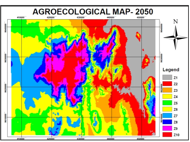
zones represented for the current data and the future data did not show a huge difference in their spatial location and pattern.
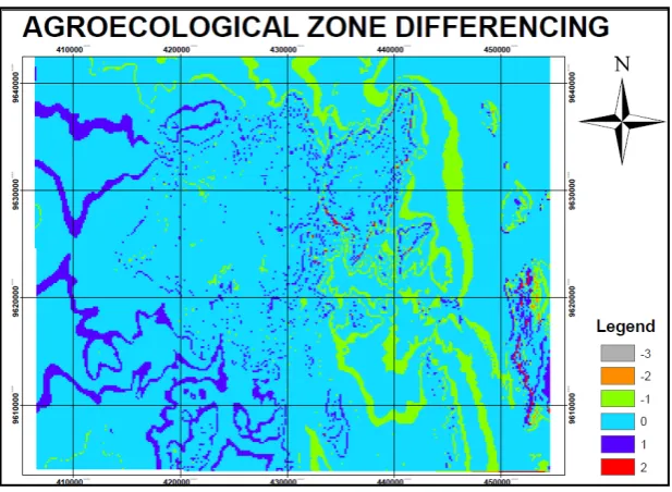
The shapes of zones had a similar characteristic. To analyze for a discrepancy (shift in zones), it prompted the need to subtract the zones by what is defined as 'image zone differencing' as illustrated in Figure 5 below. where Figure 3 was subtracted from Figure 4 (aggregated changes of all
[image:4.595.145.467.204.426.2]zones) that is to say {future zones - current zones}. The shapes of zones had a similar characteristic. To analyze for a discrepancy (shift in zones), it prompted the need to subtra d from Figure 4 (aggregated changes of all zones) that is to say {future zones - current zones}.ct the zones by what is defined as 'image zone differencing' as illustrated in Figure 5 below. where Figure 3 was subtracte
Figure 2. Existing Land Use Types for Taita Hills.
[image:4.595.148.463.446.681.2]Figure 4. Agro-Ecological Map (2050)
3.2. Zone Difference Map
Figure 5. Zone Differenced Map (Future - Recent)
The legend on Figure 5 shows the values from (-3, -2, -1, 0 +1 and +2). Zones that had an increase are shown on the legend with positive values (+) whereas those with decrease are shown with the negative values (-). The generated map of the changes can be used as a model for 'zone shift' analysis in the year 2050. Some zones in the future will reduce while others will increase. For instance, in the lower zone, where on Figure 5, we have green-colored strips, this are the (-1) values meaning there will be a reduction in zone 1, zone 2 and zone 3. On the other hand where we have blue strips on the right hand side of the same figure, the values are (+1) meaning in 2050, some of the upper zones will increase in size. Evidently seen for zone 7 in both Figure 3 and Figure 4, Zero value meant no change in the future.
3.3. Zone Description and Quantification
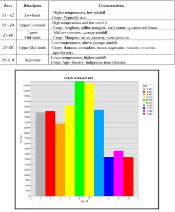
Describing the ten zones was a bit challenging but a best description was that which followed already existing AEZ by FAO. Table 2 below shows the zones and their characteristics giving suitable crops that are grown on every zone. The validity of the crops per zone was from selected field plots located on every zone. Fieldwork was done and crops found on this plots were tabulated with a GPS measurement on every crop in every plot. These data were overlaid to the classified zones in the recent AEZ case.
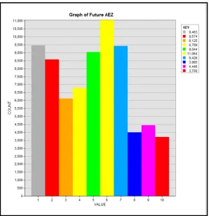
[image:5.595.151.460.341.567.2]comparisons between the zones. Quantification of the value of each zone in the current state (1960-2010) and in 2050 (future) was done. During quantification, refer to the Figures 6 and 7; Z1, Z2, Z3, Z6 and Z7 will increase in their sizes. Z4 and Z5 will unfortunately decrease but Z8, Z9 and Z10 will remain unchanged though the small changes seen are insignificant as per this study. An increase or a decrease in the zones has got a huge significance in that, a reduced or increased zone will force farmers to cultivate and or not to
[image:6.595.126.486.203.638.2]cultivate certain crops in their small subsistence farms. In an example from these results could be to narrow down to a zone where several farmers, say in zone 7, who cultivate a lot of bananas for their economy, may be affected by the 'zone shift' and perhaps put in Zone 6 where bananas do not do well due to the climate variations in that zone. A decrease in a zone will have the same impacts to the farmers just like those for an increase in a zone.
Table 2. Zone Description and Characterization
Zone Descriptor Characteristics
Z1 - Z2 Lowlands - Higher temperatures, low rainfall. -Crops: Typically sisal.
Z3 - Z4 Upper Lowlands -High temperatures and low rainfall. - Crops: Sorghum, millet, mangoes, early maturing maize and beans.
Z5-Z6 Mid-lands Lower - Mid temperatures, average rainfall - Crops: Mangoes, maize, cassava, sweet potatoes.
Z7-Z8 Upper Mid-lands -Low temperatures, above average rainfall. -Crops: Bananas, avocadoes, maize, sugarcane, potatoes, tomatoes, agro-forestry.
Z9-Z10 Highlands Lower temperatures, higher rainfall. Crops: Agro-forestry, Indigenous trees (forests).
Figure 7. Bar Graph Zone- Value Versus Count (2050)
A simple calculation that based on the widths of the zone difference result, refer to Figure 5, can be shown that about a tenth (1/10) of the total grid size is significantly a 'zone-shift'. Given that the grid size for the map is 10,000m then the shift in a zone is equivalent to 1000 meters from the map coordinates, which is equivalent to 1km on the ground. This can affect several farmers living in that region since most of them own pieces of land less than 10 hectares and majority live around the upper lowlands to upper mid-lands.
Most farmers who will be affected by these 'zone shifts' will experience a change in their cultivation patterns of some unresisting crops due to climate variations. A proper farm management practice is very essential to the farmer. With this AEZ delineation and its projection in the year 2050, the farmer and the stakeholders can be advised in advance so that they start preparing for the changes that will have impact on agricultural production and the economy at large.
4. Conclusions
It is shown that the method of multivariate clustering in conjunction with GIS is a tool that can give precise agro-ecological zone definition. Iteration is necessary to have a good delineation of a zone hence a powerful tool to analyze regions of the same climate variation in any given region and even quantify them so that the general public are informed. The government and the stakeholders on the other hand can find ways of helping farmers maintain their farm
produce and still earn a living from it. Mixed farming such as crop cultivation coupled with zero-grazing or fish farming would improve the farmers’ livelihood even with the variation of climate. It is meaningful to state that climate projections are based on physical models which are better at forecasting mean values of rainfall and temperature than their extremes. It follows that the impacts forecasted for the future represent averages of values which can sometimes strongly fluctuate from one year to another. Beyond this date (2050), and until 2100, a huge disparity exists between the scenarios because of uncertainties related to the quantities of greenhouse gases which will be actually emitted into the atmosphere, the dynamics of the agricultural sector and the agriculture’s adaptive capacity especially in Africa.
Acknowledgements
REFERENCES
[1] C. L. Williams, W. W. Hargrove, M. Liebman, Agro-ecoregionalization of Iowa Using Multivariate Geographical Clustering, Agriculture, Ecosystems and Environment , Vol. 123, 161-174, 2008.
[2] W. W. Hargrove, F. M. Hoffman, Using Multivariate Clustering to Characterize Ecoregion Borders, Computing in Science & Engineering, Vol. 1, No. 4, 18-25, 1999.
[3] C. Annmaria, D. B. Daniela, G. Giacoma, S. Fransesca, Donato. Characterization, Delineation and Visualization of Agro-Ecozones Using Multivariate Geographical Clustering, Italian Journal of Agronomy, Vol. 5,121-132, 2010.
[4] M. R. Carter M, E. G Gregorich, D. W. Anderson, J.W. Doran, H. H Jansen, F. J. Pierce. Concepts of Soil Quality and their Significance, Elsevier Amsterdam, the Netherlands, 1997.
[5] FAO. Agro-Ecological Zoning, Guidelines, Food and Agricultural Organization of the United Nations, Rome, 1996.
[6] E. E. Maeda, Agricultural Expansion and Climate Change in Taita Hills- An Assessment of Potential Environmental Impacts, University of Helsinki, 2011.
[7] R. J. Hijmans, S. E. Cameron, J. L. Parra, P. G. Jones, A. Jarvis, Very High Resolution Interpolated Climate Surfaces for Global Land Areas, International Journal of Climatology, Vol. 25, 1965-1978, 2005.
[8] Farm Management Handbook of Kenya, Volume II. Natural
Conditions and Farm Management Information. Western Kenya, 2nd Edition.
[9] F. A. Harison, O. A. Boasiako, A. Wakaitusi, T. A. Eric, Estimation of Soil Erodibility and Rainfall Erosivity Patterns Over Agro-ecological Zones of Ghana, Soil Science and Environmental Management Vol.3, No. 11, 275-279, 2012.
[10] A. A. Miguel, R. Peter, A. T. Lori, The Potential of Agro-ecology to Combat Hunger in the Developing World, A 2020 Vision for Food, Agriculture and the Environment, 1998.
[11] Land Management Component, Agro-ecosystems Analysis and Agro-ecological Zoning, a handbook, Lao-Swedish Upland Agriculture and Forestry Research Program, National Agriculture and Forestry Research Institute, Vientiane, Lao PDR, 2006.
[12] R. G. Bailey, Delineation of Ecosystem Regions, Environmental management, Vol. 7, 365-373, 1993.
[13] J. M Omernik, Ecoregions, A Spatial Framework for Environmental Management, Biological Assessment and Criteria, Tools for Water Resource Planning and Decision Making, Lewis Publishing, Boca Raton Fla, 46-62, 1995 [14] Online Available: http://www.worldclim.org/downscaling.
last access 15.07.2014.