London School of Economics and Political Science
Essays in Market Microstructure
Francesco Palazzo
A thesis submitted to the Department of Economics of the London School of
Declaration
I certify that the thesis I have presented for examination for the PhD degree of the London School of Economics and Political Science is solely my own work other than where I have clearly indicated that it is the work of others (in which case the extent of any work carried out jointly by me and any other person is clearly identified in it).
The copyright of this thesis rests with the author. Quotation from it is permitted, provided that full acknowledgement is made. This thesis may not be reproduced with-out my prior written consent.
I warrant that this authorisation does not, to the best of my belief, infringe the rights of any third party.
I declare that my thesis consists of 35,157 words.
Statement of conjoint work
Chapter 3, “Learning and Price Dynamics in Durable Goods Market”, was jointly co-authored with Min Zhang. I contributed a minimum of 50% of this work.
General decisions about the direction of research, and the proofs of the main re-sults, were made equally between the authors.
Acknowledgements
This thesis would not have been possible without the support of many people. I am very grateful to my advisors Dimitri Vayanos and Francesco Nava, for their guidance and encouragement. A special thanks goes to Andrea Prat, for his constant support and interest in my work, and for his generous invitation to Columbia University.
My work has immensely benefitted from long and fruitful discussions with my fellow PhD students. I am extremely grateful to Min Zhang and Jason R. Donaldson; they have been great co-authors and invaluable friends. Special thanks go to Markus Riegler, Ana McDowall, Oliver Pardo Reinoso, Can Celiktemur, Sebastian Kodritsch, and the other participants of the LSE Economic Theory seminar series.
I would like to thank the Bank of Italy for financial support during my PhD studies, and for a stimulating work environment now. Anatoli Segura and Taneli Mäkinen provided very valuable feedback on the work contained in this thesis.
Though there are more people who deserve thanks than I can name here, I would like to particularly thank Marco Bevilacqua, Diletta Drago, Giuseppe Calì, and Mara Giua, for sharing my enthusiastic as well as my tough moments.
Abstract
This dissertation contains three theoretical essays on the functioning and the organiza-tion of over the counter markets.
The first paper, “Is Time Enough to Alleviate Adverse Selection?,” considers a dynamic adverse selection model in which sellers pay a search cost to find a new buyer. I uncover a relationship between adverse selection and the magnitude of search costs. Interestingly, small search costs may increase the severity of the adverse selection problem, ultimately leading to a lemons market. A market design intervention may mitigate adverse selection and promote full market participation. Conditional upon an adequate level of information disclosure, a per period market participation tax, coupled with a final rebate once a seller trades, introduces a credible signalling device.
The second paper, “Peer Monitoring Incentives via Central Clearing Counterpar-ties,” studies how the novel introduction of mandatory clearing for over the counter financial assets may affect dealers’ incentives to monitor each other’s. The design of the loss allocation rules is crucial. To maximize peer monitoring incentives, a higher share of losses should be payed by surviving members with a greater trade exposure to the defaulting dealer. In practice, this mechanism can be implemented through varia-tion margin haircutting. If all members should contribute, equilibrium outcomes may be inferior to what can be achieved without clearing.
Contents
1 Is Time Enough to Alleviate Adverse Selection? 7
1.1 Introduction . . . 8
1.2 Related literature . . . 13
1.3 Model . . . 14
1.3.1 Model setup . . . 14
1.3.2 Discussion of the assumptions . . . 17
1.4 Equilibrium analysis . . . 18
1.4.1 Separating equilibria . . . 19
1.4.2 Pooling equilibria . . . 21
1.5 Welfare analysis . . . 26
1.6 Market design . . . 29
1.7 Conclusion . . . 31
1.8 Appendix A . . . 32
1.8.1 Extended notation . . . 32
1.8.2 Preliminary results . . . 34
1.8.3 Pooling equilibria . . . 39
1.8.4 Welfare analysis . . . 42
1.8.5 Market design . . . 44
1.9 Appendix B . . . 49
2 Peer Monitoring Incentives via Central Clearing Counterparties 66 2.1 Introduction . . . 67
2.2 Related literature . . . 71
2.3 Baseline model . . . 73
2.4 Equilibrium with two dealers . . . 74
2.4.1 Autarchic equilibrium . . . 75
2.4.2 Peer monitoring equilibrium . . . 75
2.4.3 Optimal CCP loss mutualization design . . . 79
2.5.1 Model . . . 83
2.5.2 Incentive compatibility forNdealers . . . 85
2.5.3 Equilibrium forN→+∞ . . . 87
2.6 Discussion . . . 94
2.7 Conclusion . . . 95
2.8 Appendix . . . 96
3 Learning and Price Dynamics in Durable Goods Markets 103 3.1 Introduction . . . 104
3.2 Information revelation and learning . . . 108
3.2.1 Model setup . . . 108
3.2.2 Public beliefs dynamics . . . 108
3.3 Dynamic auction model . . . 112
3.3.1 Trading protocol . . . 112
3.3.2 Equilibrium characterization . . . 113
3.3.3 Comparative statics . . . 114
3.4 Conclusion . . . 116
List of Figures
1.1 Equilibrium interactions with TMO. . . 22
1.2 Number of periods on the market for H-sellersκ∗(q0)and signal precisionγ. 24 1.3 Equilibria in different economiesE(γ,q0)forc≤c∗. . . 27
1.4 Efficient market intervention(τ∗,r∗). . . 31
2.1 Timing of the game.. . . 74
Chapter 1
Is Time Enough to Alleviate Adverse
Selection?
1.1
Introduction
Information asymmetry is a pervasive feature of real-world markets. Financial securi-ties, real estate, electronics and secondhand vehicles are just a few examples. One side of the market—usually buyers—lacks information or experience to ascertain the true quality of a specific good. Since Akerlof’s (1970) seminal paper, it is well known that in a static model ‘lemons’ may force high quality products out of the market.
A growing literature has been reconsidering the adverse selection problem in a dynamic environment.1 A key feature of these models is the use of time as a signalling device so that every type of seller eventually trades. In equilibrium, low quality sellers trade early while high quality sellers demand higher prices and trade afterwards. I refer to this economic mechanism as inter-temporal separation (henceforth, ITS).2 Postponing trade signals good quality, and opens up the opportunity to sell at a higher price. Although this inefficient delay among high quality sellers causes some welfare loss, eventually every seller trades.
Despite ITS theoretical importance, empirical findings seem at odds with its mech-anism. Tucker et al. (2013) point out that real estate sellers who have been on the market longer trade at lower prices, when buyers can credibly observe how long a seller has been on the market. Trading late does not seem to strengthen reputation, but instead it is perceived to signal lower quality. Furthermore, ITS fails to address Jin and Kato’s (2007) evidence on the relationship between adverse selection and market segmentation. They show that the lemons problem may induce different product qual-ities to separate between online and offline markets rather than over time. Specifically, products offered online are more likely to be of low quality, unless certified by a pro-fessional third party, while higher quality products are usually sold through the retail channel.3 Lastly, Lewis (2011) points out that greater information disclosure on eBay motors increases sellers’ chances of trading as well as final prices; nevertheless, inter-temporal separation does not explain this piece of evidence, as its mechanism works irrespective of the existence of informative signals for buyers. Together, the empirical findings of these studies suggest to reconsider—at least for some markets—how time may mitigate adverse selection in real-world markets.
This paper proposes a model to explain why these empirical patterns emerge, and how a market designer may induce high quality sellers to participate in an otherwise
1A non-exhaustive list includes Janssen and Roy (2002), Blouin (2003), Camargo and Lester (2014), Fuchs and
Skrzypacz (2013, 2014), and Kaya and Kim (2014).
2A key assumption underlying the inter-temporal separating mechanism is the ability of buyers to infer how long
a seller has been waiting on the market. They can either observe hard evidence of time on market or there is common knowledge on the initial date of the game.
3Analogously, Dewan and Hsu (2004) find that identical stamps trade at a 10–15 percent discount on eBay
lemons market. In my setup, market outcomes depend on the interaction among three main features of the dynamic sale problem. First, every seller incurs a search cost to find a new buyer and make a price offer; second, once matched with a seller, the buyer receives a binary informative signal on the specific good offered on sale; lastly, buyers may or may not have credible information on sellers’ time on market. I use the acronyms TMO and TMN to denote when time on market is observable or not. I characterize equilibria for TMO and TMN separately to understand whether revealing this information improves final allocations.
My main result is that markets with low search costs suffer from a more severe adverse selection problem. Intuitively, a low quality seller pools on the same price offered by high quality sellers because it is cheap to wait until a buyer will wrongly perceive his product as good. Due to this imitating strategy, high quality sellers may decide to stay out of such markets or, at best, to participate for a limited time only. This result is in contrast with the ITS logic, which maintains that sellers separate over time for each discount factor—a measure of search frictions—even if trading may require them to spend, on average, a long time on the market.
My main departure from models featuring ITS is an alternative assumption about the delay cost that sellers incur to find a new trade opportunity. This difference is not just a technical issue about preference specifications, as it captures two alternative economic ideas on the nature of these costs. In models with ITS, postponing trade imposes a delay cost via time discounting, reducing the present value of a positive expected payoff. Trading late is costly, but market participation always provides a non-negative payoff. In contrast, in my model postponing trade imposes a per period cost in the form of an additive utility loss and, for simplicity, there is no discounting.4,5 Sellers may stay out of the market if they expect to incur a considerable cumulative cost before trading.6 This per period cost could take many plausible forms: for example, search costs, market participation fees, maintenance costs, or in a financial market it could capture the cost of carrying an open position. For simplicity, I refer to this utility loss as a ‘search cost’ but alternative interpretations are possible depending on the market under consideration. The main point is to have an environment in which postponing trade for a sufficiently long time dissipates all gains from trade.
4I take a neutral stance and consider an equal cost for each type of seller. To the best of my knowledge, there
is no particular economic reason to assume different costs for different seller’ types. However, the main economic mechanism presented in this paper would still be valid if high quality sellers did not enjoy a significant cost advantage.
5To emphasize the different economic mechanism at work, I assume no payoff discounting. Atakan (2006)
and Lauermann and Wolinsky (2013) assume the same preference specification. Analogous results would hold if discounting has an order of magnitude sufficiently small relative to search costs; see Example 1.8.1.
6From a technical standpoint, ITS relies on discounting of an instantenous payoff. This preference specification
In my model, separation is possible when a low quality good trades at a low price that buyers always accept, whereas a high quality one trades at a higher price to the first buyer who receives a high signal on its quality. In other words, separation is based on the difference in the expected search costs of pursuing a high price strategy by the two types of sellers. More precise signals for buyers or higher search costs for sellers increase this difference. For a given search cost, higher signal precision decreases the expected cost for high quality sellers but increases the cost for low quality types. For a given signal precision, a higher search cost increases the expected cost for both types of sellers but low quality ones suffer a larger loss. Separation is possible only if high quality sellers enjoy a sufficient advantage in terms of expected search costs, i.e. if signal precision and search costs are sufficiently high.7 This separating equilibrium does not depend on whether the market exhibits TMO or TMN.
When buyers’ signals are not very informative and/or search costs are too small,8 the difference in expected search costs of a high price strategy does not prevent low quality sellers from pooling on a high price whenever possible. In turn, only two out-comes exist: either the market includes only lemons, or all sellers participate and post the same ‘high’ price, accepted only after a positive signal. A market breakdown is inevitable when the share of high quality products among the entrant sellers is below a certain threshold value, which depends on signal precision and time on market ob-servability. Specifically, a lemons market is more likely to emerge when buyers do not have sufficiently informative signals, in line with Lewis’s (2011) findings. However, my model points out a complementarity between signal precision and search costs. In this respect, the potential for a market breakdown when search costs are small may provide a rationale for Jin and Kato’s (2007) evidence on the likely exclusion of un-certified high quality sport cards from eBay.9 Online markets have almost eliminated search costs and—according to my model predictions—low types pretend to offer a high quality good, because it is cheap to wait for a buyer who receives a positive signal and accepts a high price. However, in equilibrium, prices do not convey any informa-tion on the underlying quality of the good and buyers are skeptical to accept a high price. In turn, owners of high quality goods may prefer to avoid online platforms. For example, they could either sell through an a certified intermediary, or offer a costly contractual device (for instance warranty) to alleviate adverse selection. I do not model these alternatives, but they are implicitly captured by the type-dependent reservation
7Obviously, search costs should not betoohigh; otherwise no seller would participate in the market.
8A literature on e-commerce focuses on competition and price dispersion (Clay et al. (2001) and Baye et al.
(2004)) or on market structure (Goldmanis et al. (2010)). However, to the best of my knowledge, no existing paper specifically discusses how low search costs interact with the adverse selection problem.
9However, as argued by Dellarocas (2005), eBay has been successful in solving asymmetric information problems
value that every seller enjoys. My focus is the relationship between delay costs and adverse selection; hence, I exclude other potential signalling devices.
In a pooling equilibrium—when search costs are low—information on sellers’ time on the market is crucial. It determines buyers’ prior beliefs about the likelihood of matching with a high quality seller. If time on market is observable, buyers’ prior probability of receiving a high quality good from a sellerκ periods old, say, is equal to
the share of high quality sellers in cohortκ. If time on market is not observable, buyers
hold a single prior equal to the overall share of high quality sellers in the market. The two alternative assumptions lead to different price dynamics. Because posted prices are accepted only after a high signal, under TMO the longer a seller has been on the market the lower his price offers will be: high quality goods sell more rapidly—as they are more likely to receive a high signal—and buyers realize that older sellers are more likely to offer a low quality good.10 If a seller has been on the market too long, buyers would only accept prices below the reservation value of high quality sellers who, in turn, prefer to exit the market. The model predictions of a decreasing price path and an eventual market drop out are consistent with the empirical patterns reported in Tucker et al. (2013) and Hendel et al. (2009).11
When time on market is not observable, everyone offers the same price and no seller drops out once he initially decides to participate in the market. However, high quality sellers are less likely to participate compared to the TMO case. Interestingly, under TMN neither the dynamic dimension, nor the existence of private informative signals for buyers, improves market allocations relative to a static model with unin-formed buyers. In markets with more precise signals, low quality sellers wait longer until a buyer receives a positive signal, and the pool of sellers on the market includes a larger share of low quality goods relative to the cohort of entrant sellers. This negative effect on the prior probability to receive a high quality good perfectly cancels out the positive effect of a more precise signal. In other words, under TMN, increasing signal precision is self-defeating as it worsens the average market quality which, in turn, de-termines buyers’ prior expectations of receive a high quality good. Thus, the ability to observe time on market may improve welfare when the number of high quality goods is low.
In light of these negative results, I perform in section 1.6 a market design exercise for the limit case of zero search costs. I analyze whether a system of transfers condi-tional on market participation and trade may alleviate adverse selection and promote
10Taylor (1999) is the first paper to exploit this social learning mechanism in the context of a two-period adverse
selection model (see section 2.2).
11Hendel et al. (2009) document that some real estate sellers in Madison, WI decide to switch to a realtor after
full market participation. I focus on mechanisms that satisfy a series of properties: budget balance, informational efficiency of prices, and interim individual rationality. The efficient market design intervention achieves separation through a constant market participation tax, and it relaxes sellers’ individual rationality constraint through a final rebate conditional on trade. A low quality seller does not find it profitable to post a high price because, on average, he is less likely to find a buyer who receives a high signal; if he pursued a high price strategy, he would pay, on average, a cumulative amount of market participation taxes that would make imitation unprofitable. In terms of incentive compatibility constraints, the market participation tax is analogous to a per period search cost. Nevertheless, the former is not a waste of economic resources, and it can be partially recouped through a rebate, relaxing sellers’ market participation constraints. Although time on market observability plays a relevant role in all pooling equilibria, it doesnot affect the efficient mechanism. Taxes and rebates are inversely proportional to buyers’ signal precision, but they do not depend on sellers’ time on market, although in principle they could. This efficient market design intervention achieves full market participation in a large set of economies, but it is not successful when buyers’ signals are close to being uninformative.
From a technical standpoint, the model is a dynamic signalling game since in every period the informed party—sellers—decides to post the price at which they are willing to trade. In previous non-stationary models, the bargaining protocol either assumes exogenous prices12 or buyers make take-it-or-leave-it offers.13 As in the Diamond’s (1971) paradox, the latter protocol implicitly fixes the price at which high quality sell-ers trade—equal to their exogenous reservation value—and only the price accepted by low quality sellers is determined endogenously. In my setup, this bargaining solution leads to a hold-up problem: high quality sellers would not pay a search cost to trade at their reservation value. I assign all bargaining power to sellers to improve their chances of participating in the market. Equilibrium characterization is challenging because I have to take into account—for every cohort of sellers—an endogenous behavioural strategy (possibly mixed) for each type of seller.
In the next section I discuss the related literature. Section 3 presents the model setup. Section 4 characterizes the equilibria when search costs are close to zero. Sec-tion 5 discusses the welfare properties of equilibria. SecSec-tion 6 derives the efficient intervention. Section 7 concludes. All proofs are in Appendices A and B.
12See Wolinsky (1990), Blouin (2003) and Camargo and Lester (2014).
1.2
Related literature
This paper is mainly related to the theoretical literature on dynamic adverse selection in decentralized markets.14 Two different types of goods coexist in the same market, but product quality is sellers’ private information. The literature mainly considers non-stationary equilibria, as the market starts at an initial date and strategies depend on time.15 Analogously, the TMO case in this paper leads to a non-stationary equilibrium, since sellers’ strategies generally depend on previous time on market. In my setup, time on market coincides with the number of previous matches with buyers.16,17
Blouin (2003), Camargo and Lester (2014), and Moreno and Wooders (2014) char-acterize non-stationary equilibria in infinite horizon games.18 Inter-temporal separa-tion allows all sellers to trade over time. The main differences among these papers have to do with the division of trade surplus and are partly driven by alternative bargaining protocols. The former two papers adopt the exogenous price bargaining of Wolinsky (1990), while the latter assume buyers make take-it-or-leave-it offers. Kaya and Kim (2014) construct a model in which buyers receive private informative signals and make offers to sellers. In their setup, prices and beliefs converge to a steady state, and the transition depends on the initial probability of trading with a high quality seller: if it is high, prices and beliefs move downward as in Taylor (1999); if it is low, ITS kicks in and allows sellers to separate. As discussed in section 2.3, I assume sellers make take-it-or-leave-it offers. In contrast to what happens in Moreno and Wooders (2010, 2014) or Kaya and Kim (2014), a hold-up problem would arise in my setup if H-sellers could only trade at their reservation value vH. This is not a concern in models that use dis-counting of an instantaneous payoff: in equilibrium high quality sellers discount a zero payoff as they trade at their reservation value. My TMO setup is a non-stationary dy-namic signalling game with endogenous prices, and the main challenges arise because H-sellers’ posted prices are generally non-constant over time.
14The latter term defines a class of models that depart from the classic Walrasian price formation paradigm to
explicitly model the bilateral interaction between buyers and sellers. A non-exhaustive list of previous papers on decentralized markets with complete product information includes Diamond (1971), Rubinstein and Wolinsky (1985), Gale (1986a,b), Duffie et al. (2005, 2007), Vayanos and Weill (2008), and Lagos and Rocheteau (2009). Wolinsky (1990) considers a decentralized market with asymmetric information on the common quality of all units. Serrano and Yosha (1993), Blouin and Serrano (2001), and Duffie et al. (2009, 2014) provide other contributions to this literature.
15Daley and Green (2012) analyze a dynamic setting in which buyers receive public information on the asset value
at random arrival times. Buyers may enter a waiting period: if good news arrives confidence is restored and the market reopens; otherwise, there is a partial sell off of low value assets.
16I prefer to use the expression ‘time on market’ for lexical convenience.
17Kim (2014) shows that when market frictions are small (small discount rate), observing only time on market
is welfare-improving relative to public information of previous matches. This result stems from the fact that staying on the market strengthens reputation; in this respect, information on previous matches conveys a more precise signal than time on market. As a consequence, sellers tend to delay trade as they reject price offers more often. However, my paper points out why this ITS mechanism might not work, and it shows that—when search frictions are small— a longer stay on the market is interpreted as a negative indicator of quality. Therefore, in my setup the welfare comparison between the two regimes could be reversed.
My paper is also related to a new strand of literature on optimal market intervention for lemons markets. Fuchs and Skrzypacz (2013) study how to minimize delay costs through the optimal design of market openings. Fuchs and Skrzypacz (2014) consider government interventions through taxes and subsidies.19 Their Pareto improving bud-get balanced policy suggests a short tax exempt trading window followed by a short lived period of positive taxes; sellers trade immediately and after the tax goes back to zero. My efficient intervention also points out the need to subsidize initial trade, but it prescribes a constant market participation tax thereafter (see section 1.6). Fuchs and Skrzypacz’s (2014) short-lived taxation policy would not be effective in my setup by the same logic that excludes ITS.
My results are also related to the literature on sequential trading between a long-lived seller and a sequence of short-long-lived buyers. Taylor (1999) considers a two-period model in which a single informed seller posts prices under different price observability assumptions.20 His paper was the first to point out the negative informational exter-nality that affects older cohorts of sellers when buyers observe private informative sig-nals. Lastly, Lauermann and Wolinsky (2013) consider a sequential search model with TMN, informative private signals for buyers, and additive search costs. They show the existence of a search friction that reduces price informativeness compared to a com-mon auction environment. They consider buyers who receive signals sampled from a continuous distribution—possibly of unbounded precision—while I use a simple sym-metric binary signal of bounded precision. My choice is motivated by tractability concerns, especially for the non-stationary equilibria under TMO. Moreover, I focus on allocative efficiency and market exclusion, while they analyze informational effi-ciency.
1.3
Model
This section presents the model setup and discusses how the main assumptions relate to the research questions.
1.3.1
Model setup
Consider a decentralized market where trade is possible only in bilateral transactions between one buyer and one seller.21 Each seller is endowed with a single indivisible
19Their paper differs from Philippon and Skreta (2012) and Tirole (2012) because the latter consider a
governe-ment intervention in the presence of a static competitive private market.
20Hörner and Vieille (2009) and Fuchs et al. (2014) also study the effect of price history observability in models
in which buyers have no informative signals.
good of high (H) or low (L) quality. A seller knows the quality of his product but nobody else can observe it. Letθλ andvλ be buyers and sellers’ valuation, respectively,
for a product of qualityλ ∈ {H,L}, and assumeθH>vH>θL >vL. I use the terms H-sellers and L-sellers to refer to sellers with goods of high and low quality.
Time t ∈ {..,−1,0,1, ..} is discrete and in each period a set of sellers µt of unit mass is born. Only a fractionq0∈(0,1), independent oft, of newly born sellers owns a high quality good. Sellers are long lived and they can participate in the market until they trade or exit. Buyers live for a single period and they always outnumber sellers.
I denote the set of sellers participating in the market at timet asSt, whileSκ t ⊂St is the set of sellers who have been participating in the market for κ ∈N0 previous
periods; similarly, Sκ λ,t ⊂S
κ
t is the subset of sellers of type λ in Sκt .22 Sellers pay a search cost c to participate in the market and match with a buyer. Buyers match uniformly at random with sellers and have no search cost. For simplicity, they have no opportunity to buy a good and re-sell it on the market. All players are risk-neutral and have quasi-linear utilities with respect to monetary transfers. Sellers do not discount future payoffs.
Buyers and sellers trade according to a simple mechanism. Each selleri∈St−1∪µt who has not traded at time t−1 takes an action aS,i ∈ AS= {{D},R+}, where D
denotes the decision to irreversibly drop out of the market, and p∈R+ is the posted
price at which he commits to sell the good in period t. If aS,i= D, seller i is not matched with a buyer and does not pay the costc; however, he has no future possibility of participating in the market. IfaS,i=p, selleripayscand gets matched with a buyer. A particular history for seller i∈Sκ is indicated with hκ
i = (hκ
−1
i ,aκS,i×aκB,i) (with h−i 1=∅) andHκ is the set of all possible histories.
LetZκ
i ⊂Hiκ denote the set of terminal histories for selleriafterκ previous periods (with Zi= S
κ∈N0
Zκ
i ). If hκi ∈Ziκ selleri exits the market after κ previous periods in the market and he cannot choose any further action, i.e. ASj,i =∅, j ≥κ+1. Let
Zκ
i (D)⊂Ziκ include all terminal histories in which seller i drops out of the market after κ periods; similarly, Ziκ(p)⊂Ziκ denotes the set of histories in which seller i
trades at price p after κ previous periods in the market. The final payoff to seller
i∈Sκ
λ,t inz∈Z κ i is
˜ uλ(z) =
(
−κc ifz∈Ziκ(D)
p−vλ−(κ+1)c ifz∈Ziκ(p)
Once matched with seller i, a buyer receives a private signal ξ ∈ {H,L} on his 22To simplify exposition, I slightly abuse notation usingS,Sκ,Sκ
λto denote both the set or the measure of sellers
product quality, but she cannot observe his previous price history.23 Buyers’ sig-nals have precisionγ ∈(12,1), i.e. PH(ξ =H) =PL(ξ =L) =γ. For a given vector
(θH,vH,θL,vL), I parametrize a specific economyE(γ,q0)by signal precision γ and newly born measureq0of H-sellers.
I consider two different setups for publicly available information. If time on market is observable (TMO), a buyer observes how long a seller has been participating in the market; i.e. it is common knowledge whetheri∈Sκ
t for someκ ∈N0. In contrast, if
time on market isnotobservable (TMN) no buyer can observe this information. When time on market is observable, a buyer’s information setIB(p,κ,ξ)includes the seller’s offer p, his previousκ periods in the market, and the buyer’s signalξ. If
time on market is not observable, it only includes pandξ (i.e. IB(p,ξ)). Given her information set, a matched buyer takes an actionaB,i∈AB={A,R}, whereAdenotes acceptance andRrejection of the selleriprice offer. If she accepts offerp, trade occurs and they leave the market; if she rejects, no exchange takes place and sellerimoves to periodt+1.
In this paper, I only consider stationary and symmetric equilibria of the game. Players’ equilibrium strategies do not depend on timet, but only on seller’s typeλ,
cohort κ and history hκi−1. In this class of equilibria, the mass of sellers St, Stκ and Sκ
λ,t is constant over time—i.e. St =S, S κ
t =Sκ and Sκλ,t =S κ
λ for everyκ ∈N0 and
t ∈Z—and I omit the subscriptt in the remainder of this paper. I denote with σ a
strategy profile and withπ a belief system. A strategy profileσ and a belief systemπ
form an assessment (σ,π). I use σ−i and π−i to indicate the strategy profile and the belief system of any agent other thani.
Letqκ =
P(θH|Sκ)be the prior probability under uniform random matching that a seller inSκ offers a high quality good. On the equilibrium path, a buyer incorporates
her private signal into the publicly available information according to Bayes’ rule.
Definition 1.3.1 A assessment (σ,π) is an equilibrium of the game if it is a weak
Perfect Bayesian Equilibrium (PBE) with the following restrictions:
1. Stationarity:buyers and sellers in Sκ
λ,tand S κ
λ,t0play identical strategies∀t6=t
0.
2. Symmetry:if sellers i,j∈Sκ
λ have h κ−1
i =h κ−1
j , they play the same strategy.
3. Pure strategies: buyers only play pure behavioural strategies.
I impose a few restrictions on the notion of weak PBE.24 First, strategies do not depend on timet for otherwise identical sellers. Second, sellers’ strategies can differ
23This assumption significantly simplifies the set of possible equilibria. See Taylor (1999), Hörner and Vieille
(2009) and Fuchs et al. (2014) for models that consider equilibria with price history observability.
only with respect to seller’ types λ ∈ {H,L}, cohorts Sκ
λ and previous history h κ−1
i . The third condition restricts buyers—conditional on an information set—to play pure strategies,25 but sellers can use mixed strategies.
In Propositions 1.4.3 and 1.4.4, I use the undefeated equilibrium refinement intro-duced by Mailath et al. (1993).26 I adopt this refinement for two simple purposes: (i) to rule out the self-fulfilling PBE in which only L-sellers trade because buyers believe only L-sellers participate, whenever there exists another PBE in which H-sellers par-ticipate in the market; and (ii) to select among the set of pooling PBE the one with the highest possible prices, i.e. pκ =
EπB[θ|IB(p
κ,·,H)]. Therefore, it isnotused to
rule out separating or semi-separating strategy profiles, differently from what happens in the Spence (1973) model.27 Indeed, Lemma 1.4.1—the main characterization result for smallc—does not rely on the undefeated refinement to show that the only admissi-ble behavioural strategies have both types of sellers inSκ pool on the same price. De
facto the undefeated refinement is not restrictive, but instead is a conservative choice to illustrate that a market breakdown is still possible under a dynamic setup. Indeed, this refinement selects the equilibrium in which H-sellers’ market participation constraint is satisfied for the lowest possibleq0.28
For simplicity, I do not specify out-of-equilibrium beliefs in the proposition state-ments. The main result on the admissible equilibrium strategies—Lemma 1.4.1—rules out other strategies without relying on any specific out-of-equilibrium belief. The re-sulting admissible equilibria only require buyers to hold sufficiently pessimistic beliefs out of the equilibrium path.
1.3.2
Discussion of the assumptions
I briefly discuss the main model assumptions and how they relate to the literature.
Additive search cost c.My main departure from the previous literature—with the notable exception of Lauermann and Wolinsky (2013)—is the introduction of a search cost. It can be alternatively interpreted as an additive and symmetric specification of delay costs. This preference specification has two main properties: (i) sellers stay out of the market if they expect to trade after a long time, since the cumulative amount of search costs would be larger than their total gains from trade; and (ii) all sellers suffer the same utility loss if they postpone trade.29 Additive delay costs are not the only
25Buyers’ strategies depend on the information set, and this restriction does not prevent strategies to depend on
signalξ despite the latter may not change the beliefπB. To understand the logic of this restriction see footnote 35.
26See Definition 1.8.2 in the Appendix for a formal definition. 27See Mailath et al. (1993) for a discussion.
28Roughly speaking, H-sellers inSκparticipate only if
EπB[θ|IB(p
κ,·,H)]≥pκ≥v
H, and, in a pooling equilibrium,
this expectation is strictly increasing inπB, which, in turn, is weakly increasing inq0.
preference specification with these properties,30but I prefer an additive cost because it can be easily interpreted as a search cost. Moreover, it provides a natural starting point for my market design exercise in which transfers enter utility additively.
Bargaining protocol. All previous papers in the literature adopt a specific bar-gaining protocol to make the model tractable. Blouin (2003) and Camargo and Lester (2014) adopt the exogenous price bargaining protocol first introduced by Wolinsky (1990). Moreno and Wooders (2010) and Kaya and Kim (2014) assume that buyers make take-it or leave-it offers; Lauermann and Wolinsky (2013) use a random propos-als bargaining model to avoid dealing with out of equilibrium beliefs. In this paper, sellers—the fully informed party—make take-it-or-leave-it offers to buyers. In addi-tion to being a realistic assumpaddi-tion in many real-world markets, this trade protocol gives full bargaining power to sellers. Since high quality sellers may stay out of the market, this assumption seems a conservative benchmark for assessing when their mar-ket exclusion is more likely.
Short-lived buyers. Buyers are exposed only to the idiosyncratic risk of buying a lemon. There is no aggregate uncertainty as in Wolinsky (1990) or Blouin and Serrano (2001), in which all units of the good have the same quality and the main trade-off for buyers is between delaying trade to acquire more information or trading early at a po-tentially larger loss. In my setup, short-lived buyers are not essential to the main model insights and they simplify exposition. Moreover, a long-lived buyer may extract some trade surplus as his bargaining position is likely to strengthen. As for the bargaining protocol, I assume short-lived buyers because it seems a conservative choice to study when high quality sellers are more likely to stay out of the market.
1.4
Equilibrium analysis
Before presenting the main results in sections 1.4.1 and 1.4.2, I restrict attention to economies in which the temporal dimension may help to alleviate the adverse se-lection problem. Formally, I do not consider economies where all sellers can trade immediately, because no allocative efficiency problem arises. It is straightforward to realize that this equilibrium outcome exists only if all sellers post a price p and buy-ers always accept. In this pooling equilibrium, (i) buybuy-ers accept p even whenξ =L,
and (ii) high quality sellers find it profitable to participate in the market. This equi-librium requires p≤EπB[θ|IB(p,0,L)]and p≥vH+c. These two conditions imply
30For example, it is also the case forδκp−v
λ, a utility specification that can be easily interpreted as a seller who
EπB[θ|IB(p,0,L)]≥vH+c, or:
q0≥ γ(vH+c−θL)
(1−γ)(θH−vH−c) +γ(vH+c−θL)
:=qIPc 31
The highest possible pooling price, p =EπB[θ|IB(p,0,L)], is decreasing in γ;
henceqIPc is increasing inγ. The intuition is straightforward: immediate trade requires
buyers to accept when ξ =L, and a more informative signal has a stronger negative
impact on the posterior expectation. Buyers pay at least vH+c when they receive
ξ =Lonly if they hold a sufficiently high prior probabilityq0of matching with a high
quality seller.
I also refer to another relevant quantity: the minimum value ofq0above which all sellers trade in a static version of the model withnoinformative signals. As this is sim-ply Akerlof (1970) model with an initial search costc, it is easy to conclude all sellers trade only ifq0≥ vH−θL+c
θH−θL :=q
S
c. This quantity is a benchmark for understanding how the temporal dimension may improve market outcomes relative to a static model. In the remainder of this paper, unless specified, I assumeq0<qSc.
1.4.1
Separating equilibria
A first natural question concerns the existence of a separating equilibrium. The litera-ture shows that it is possible for sellers to separate overtime. In this respect, waiting is a signalling device analogous to education in the classic Spence (1973) model. Buyers find this separating mechanism credible, and they are willing to pay higher prices for sellers who have been on the market longer. Importantly, inter-temporal separation works even when buyers do not have any informative signal (γ = 12).
A few common assumptions make ITS possible: (i) sellers’ delay costs enter utility through discounting (at rate δ <1); (ii) there exist strictly positive gains from trade
for all types of goods; and (iii) sellers discount an instantaneous payoff as sale and production occur contemporaneously, or goods are durable.32
Assumption (i), (ii) and (iii) lead to a preference specificationδκ(p−vλ)whenever
a seller trades afterκ previous periods in the market. For a utility functionu(λ,κ,p),
the strict single-crossing condition is satisfied if up(λ,κ,p)
|uκ(λ,κ,p)| is strictly increasing in λ
and it has the same sign for all (λ,κ,p) (see Milgrom and Shannon (1994)).
Pay-off discounting has u(λ,κ,p) = δκ(p−vλ), and the ratio of partial derivatives is
δκ
|(p−vλ)δκlnδ|, is always positive and is strictly increasing in λ as vH >vL. In con-31The subscriptcindexes threshold values forq0to the search costc. Later I useqIP
0 to denote the value of the
threshold forc=0.
32A durable good provides a per period flow utilityyto its owner, so it is worth y
1−δ to the seller. Alternatively,
trast, in my modelu(λ,κ,p) =p−vλ−(κ+1)cand this ratio is equal to 1c. Similarly,
ifu(λ,κ,p) =δκp−vλ, then |p δκ
δκlnδ| is constant for allλ. The last specification
de-scribes an economy where sellers pay the production cost before market participation. Payoff discounting of an instantaneous payoff—as used in models with ITS— makes sellers’ individual rationality constraint redundant. As long as they can trade at a price greater or equal to their reservation valuevλ, they can wait indefinitely since
δκ(p−vλ)≥0. Indeed, previous models share the feature that H-sellers only trade at
p=vH, de facto eliminating their temporal preferences. This property is crucial for ITS; in fact, high quality sellers accommodate any period of delay deemed necessary to prevent low quality sellers from deviating.33 Final allocations are inefficient because some sellers delay their trades, but all sellers eventually trade.
In my setup the ITS mechanism is not possible without informative signals.
Proposition 1.4.1 Assume time on market is observable and buyers have no signals. For every c>0an inter-temporal separating equilibrium does not exist.
Intuitively, time could credibly signal higher quality only if H-sellers incur a cumu-lative utility loss larger than all gains from trade for high quality goods. Therefore, market participation is no longer profitable, and they prefer to stay out of the market. Formally, the incentive compatible delay period leads to a utility loss, which violates the individual rationality constraint of H-sellers.34
Nonetheless, separation is possible thanks to the combined effect of buyers’ infor-mative signals and search costs. I first introduce a notion of separating equilibrium.
Definition 1.4.1 An equilibrium assessment is separating if H- and L-sellers post dif-ferent prices after every history hκ
i ∈Hκ and buyers accept with positive probability.
Proposition 1.4.2 characterizes the unique separating equilibrium of the game.
Proposition 1.4.2 Irrespective of time on market observability, a separating equilib-rium exists if and only if
c∈
1−γ
γ (θH−θL),γ(θH−
vH)
In equilibrium, high quality sellers post θH and low quality sellers post θL. Buyers acceptθH only after a high signal, but they always acceptθL.
33A hybrid model with search costscand payoff discounting
δ<1may or may not admit the existence of an ITS
equilibrium. For everyc, it is possible to find aδ sufficiently close to 1 such that ITS is not possible; see Example
1.8.1 in Appendix A. I focus on theδ=1case because it provides a neat characterization of the results and a sharp intuition of the underlying economic mechanism.
34The impossibility of this result depends on the additive specification of delay costs, and it is unchanged even if
A separating equilibrium exists when both search costs and signal precision are sufficiently high. If signal precision is too low, the interval in Proposition 1.4.2 does not exist. A low quality seller does not postθH, and wait until a buyer receives a high signal, because he expects to pay too high a search cost compared to the immediate payoff of revealing his type and trading at a lower price θL. On average, H-sellers receive a high signal after 1γ periods, while L-sellers do so after 1−1γ periods; as a result, informative private signals create an asymmetric cost of delay between seller’ types. Importantly, no separating equilibrium exists when signals are uninformative (γ= 12). In other words, differences in the probability of receiving a high signal restore
a single-crossing condition and allow separation. The temporal dimension is a neces-sary condition, but it contributes to the creation of a credible signalling device only with sufficiently informative signals and an adequate level of search costs.35
1.4.2
Pooling equilibria
This section provides a complete characterization of equilibria when the search cost is close to zero. I separately analyze each public information setup—TMO and TMN— although the underlying economic intuition is similar.
When c is small, low quality sellers have strong mimicking incentives. Lemma 1.4.1 states the admissible behavioural strategies on the equilibrium path.
Lemma 1.4.1 There exists c∗ >0 such that for every c≤c∗ every equilibrium path only admits the following behavioural strategies for sellers in Sκ:
• TMO and q0<qSc:
– H- and L-sellers post a price pκ that buyers accept only after a high signal.
– H- and L-sellers only post prices rejected with probability one.36
– H-sellers stay out of the market and L-sellers trade at priceθL.
• TMN and q0<qIPc :
35Proposition 1.4.2 is a pure strategy PBE. Definition 1.3.1 allows mixed strategies for sellers, but it excludes
them for buyers. If buyers could play mixed strategies, it is easy to show that a separating equilibrium in mixed strategies would exist for allc>0if and only ifγ≥2θθH−θL+c
H−vH−θL+c>
1
2. After receiving a high signal, buyers should play
a specific randomization between accepting or rejectingθH. A lower search cost requires a higher rejection probability.
However, this mixed strategy equilibrium does not have a very realistic flavour. It suggests that in real-world markets buyers play sophisticated randomizations with the sole purpose of helping to separate sellers. Keeping in mind this theoretical possibility, I prefer to focus on equilibria in which buyers play pure strategies and separation is mainly determined by sellers’ behaviour, search costs, and the information structure. Lastly, even with mixed strategies, separation is not possible in the limit case ofc=0, while the equilibria in section 1.4.2 continue to exist.
36This case is not interesting, and it is a pathological result of signalling games. The PBE notion allows for
these ‘sudden stops’ in trade when buyers hold pessimistic beliefs on sellers in cohortSκand accept only ifp≤θL; in
κ ξ
Buyer
Sellerλ
Pλ[trade] qκ+1
Vκ+1
λ
σB
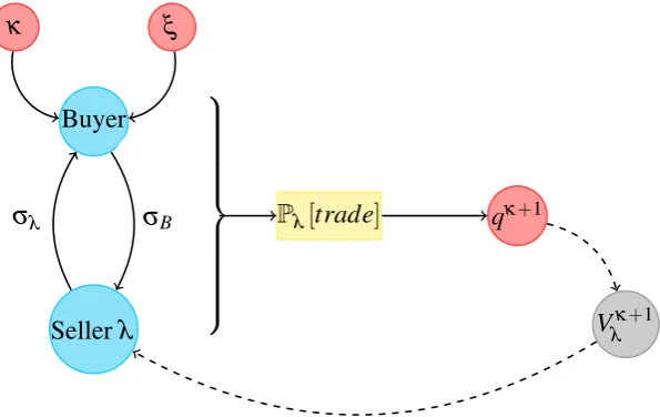
[image:24.595.172.470.81.269.2]σλ
Figure 1.1:Equilibrium interactions with TMO.
– H- and L-sellers post a pricep that buyers accept only after a high signal.¯ – H-sellers stay out of the market and L-sellers trade at priceθL.
Irrespective of time on market observability, if H-sellers participate in the market— posting a price accepted with positive probability—equilibria are possible only in pool-ing strategies.37 Both types of seller offer the same price and buyers accept only if they receive a high signal. When time on market is observable, prices may be different among different cohorts of sellers, but they post a unique price when this information is not available.38 Even if a low quality seller is unlikely to receive a high signal, this event has a strictly positive probability 1−γ >0. Low search costs reduce the cost of
finding a new buyer, and low quality sellers find it profitable to demand a high price, looking for a buyer who receives a wrong signal. If they happen not to sell at a high price, they can always reveal their type and trade at θL. The absence of a credible signalling device precludes separation, and different types of sellers pool on the same action.
Lemma 1.4.1 helps to characterize the set of equilibria of this dynamic signalling game; in the TMO case, the model is non-stationary because equilibrium strategies may depend on κ. Indeed, this dynamic game cannot be solved recursively, as
cur-rent strategies depend on future continuation values and, viceversa, the latter generally depend on the former because they endogenously determine the share of high quality sellers in each cohort. Figure 1.1 represents this equilibrium interaction between cur-rent strategies and future continuation values. To further illustrate this point, consider how buyers form expectations. First, they have a prior probability of being randomly
matched with a high quality seller inSκ. In equilibrium, this prior is determined
en-dogenously and is equal to the share of H-sellers in cohortSκ because of uniform
ran-dom matching (i.e. qκ =SκH
Sκ). Once matched with seller, a buyer observes his age and
posted price, and she updates her beliefs according to signalξ. The valueqκ plays a
substantial role in forming expectations, and it contributes to determine the maximum price that buyers accept from a seller belonging to cohort Sκ. In turn, equilibrium
prices determine whether H-sellers want to participate in the market, while equilib-rium strategies determine the type-dependent trade probabilities and the evolution of qκ across different cohortsSκ.
Due to Lemma 1.4.1, the set of admissible behavioural strategy is tractable—either a pooling price accepted after a high signal or only L-sellers trade—and the equilib-rium characterization is straightforward. The next two subsections illustrate how final market outcomes depend on time on market observability.
Time on market observability
Time on market observability (TMO) refers to buyers’ ability to observe how long each seller has been participating in the market. Although this information is specific to each individual seller, it plays a crucial role in shaping overall market dynamics. The model provides a tractable framework to analyze how the bilateral asymmetric information problem affects aggregate market dynamics and—reciprocally—how market dynamics influence the possible terms of trade in bilateral transactions.
Proposition 1.4.3 characterizes the unique undefeated equilibrium of the game for csufficiently small.
Proposition 1.4.3 Let q0<qSc. There exists c∗>0such that∀c≤c∗there is a unique undefeated equilibrium.
1. If q0≥qOc := (1−γ)(
vH+cγ−θL)
γ(θH+cγ−vH) + (1−γ)(vH−θL−γc)
• Forκ ≤κ∗(q0)<∞, κ∗(q0) =maxκ∈N0:qκ ≥qOc , H- and L-sellers in Sκ post
pκ =
EπB[θ|IB(p
κ,
κ,H)]
and buyers accept if and only ifξ =H.
0 1 2 3 4 5 6 7 8 9 0
0.1 0.2 0.3 0.4 0.5 0.6 0.7
κ
q
κ
γ= 0.5 7 5
γ= 0.7
γ= 0.8 2 5
[image:26.595.185.461.88.248.2]γ= 0.9 5
Figure 1.2: Number of periods on the market for H-sellersκ∗(q0)and signal precisionγ.
• Forκ<κ∗(q0)the share of H-sellers across different cohorts is decreasing
inκ:
qκ+1= (1−γ)q κ
(1−γ) + (2γ−1)(1−qκ)
2. If q0<qOc only L-sellers participate in the market and trade at priceθL.
Proposition 1.4.3 proves the existence of a unique undefeated equilibrium for suf-ficiently smallc. All sellers from cohortSκ post the same price pκ, and buyers accept
only if they receive a high signal ξ =H. H-sellers are more likely to trade and, on
average, they exit the market more rapidly than L-sellers. Thanks to the law of large numbers,qκ can be expressed as the solution of a first order difference equation. The
share of H-sellers is decreasing in κ: the longer a seller has been on the market, the
lower buyers’ prior belief to match with a high quality seller. Once this belief falls below the minimum threshold qOc, no buyer would be willing to pay a price above H-sellers’ reservation utility, and the latter prefer to drop out of the market.
Taylor (1999) is the first to point out a negative price externality on older cohorts of sellers. Recently, Kaya and Kim (2014) obtain a similar dynamic when the initial prior belief in meeting a high quality seller is sufficiently high. Proposition 1.4.3 suggests a declining price pathanda decision to exit the market after a finite number of periods. No market dropout occurs in Taylor (1999) or Kaya and Kim (2014). My result differs from Kaya and Kim’s when the prior probability is low (q0 <qOc): they predict a dynamic closely related to the ITS mechanism, while Proposition 1.4.3 suggests that H-sellers stay out of the market.
Greater signal precision γ leads to a more rapid decrease in qκ (see Figure 1.2).
However,γ’s effect on the measure of H-sellers that exit the market without trading is
H-sellers who trade in every periodκ ≤κ∗(q0).
Time on market not observable
Even when time on market is not observable, for smallcLemma 1.4.1 guarantees that all sellers post the same price and buyers accept only if they receive a high signal. Buyers do not distinguish sellers’ cohorts, so their prior belief in matching with a high quality seller does not depend onκ and is equal to the share of H-sellers in the overall
market. In a stationary equilibrium, this share does not change over time because the mass of each type of seller is constant, i.e. ¯qt=q¯andSκλ,t=Sκλ for everyt andλ. This
is possible if and only if the entry and exit flows are equal for each type. The entry and exit conditions impose a pair of equations that jointly determineqand the overall measure of sellers, sayS.
H-sellers: q0=Sγq
L-sellers: (1−q0) =S(1−γ)(1−q)
The following proposition describes the equilibrium.
Proposition 1.4.4 Let q0<qIPc . There exists c∗>0such that∀c≤c∗there is a unique undefeated equilibrium.
1. If q0≥qNc :=
vH−θL+cγ
θH−θL
>qSc
• Both types of sellers post price
pk=p=EπB[θ|IB(p,H)] =q0θH+ (1−q0)θL
for allκ ∈N0and buyers accept if and only ifξ =H.
• In every period
¯
S= γ−q
0(2γ−1)
γ(1−γ)
q= q
0(1−γ)
γ−q0(2γ−1) <
q0
2. If q0<qNc only L-sellers participate in the market and they trade at priceθL.
Similar to Proposition 1.4.3, H-sellers do not participate in the market when their initial share is too small (q0<qNc). In comparison to the TMO case, they participate in the market for a smaller set of economies as the thresholdqNc is strictly higher than qOc.39 If the initial share of high quality sellers is sufficiently high, all sellers post
39Precisely, this holds when c
γ<θH−vH. This is a necessary condition to haveq
a unique price p irrespective of their previous periods in the market. Sellers are not penalized if they trade late, because buyers do not observe previous time on market, and they hold a single prior probability ¯q. If a high quality seller participates in the market, he will continue to do so until he trades. This result follows directly from the forward-looking maximization problem and the fact that previous search costs are sunk.
The equilibrium share of H-sellers ¯qis strictly lower thanq0. The underlying eco-nomic intuition is simple: on average, H-sellers trade before L-sellers (1
γ versus
1 1−γ
periods, respectively); the latter stay longer on the market and decrease H-sellers’ mar-ket share below q0. The value of ¯qis negatively related to signal precisionγ because
it decreases the average time on market for H-sellers and increases it for L-sellers. The negative impact of γ on ¯q perfectly outweighs the positive effect that a higher
signal precision has on buyers’ posterior beliefs after ξ =H. This feedback effect
makes signal precision irrelevant for equilibrium prices; in fact, the pooling price p =q0θH+ (1−q0)θL does not depend on γ. In particular, it is equal to buyers’
expected value for a good offered by newly born sellers (S0)beforereceiving a signal. Whenγ > 12 all sellers trade immediately only ifq0≥qIPc >qSc. Proposition 1.4.4 implies that H-sellers participate only ifq0≥qNc >qSc. Therefore, for small cneither the temporal dimension nor buyers’ informative signals mitigate the adverse selec-tion problem. Actually, because qNc >qSc, all sellers trade for a strictly smaller set of economies compared to the classic static adverse selection model (althoughqN0 =qS0). Janssen and Roy (2004) point out that the infinite repetition of the static equilibrium is the only stationary equilibrium of a dynamic adverse selection model with uninformed buyers. Proposition 1.4.4 suggests that this result also applies when buyers have infor-mative signals. Even though this conclusion seems extreme, the mechanism in place is suggestive and it might be worth assessing its empirical validity.
1.5
Welfare analysis
In this section, I first study how different information structures compare in terms of welfare. Then, I discuss how a smallcmay actually reduce H-sellers’ market partici-pation compared to a situation with higher costs.
Definition 1.5.1 introduces a simple notion of allocative efficiency that does not take into account how many periods elapse before sellers trade.
In my model setup with transferable utility, it is natural to adopt a utilitarian wel-fare criterion. Clearly, if an equilibrium is not allocative efficient then it does not maximize total welfare. As there is no time discounting, ifc&0 an allocative efficient equilibrium is arbitrarily close to maximize utilitarian welfare. Moreover, since the transfer scheme is budget balanced—prices paid by buyers are equal to prices received by sellers—a utilitarian allocation is also Pareto efficient.
Proposition 1.5.1 summarizes the welfare properties of equilibria in the relevant set of economies withq0<qSc.
Proposition 1.5.1 Let q0<qSc. The following statements hold when c&0:
1. No equilibrium allocation maximizes total welfare.
2. If q0∈
qO0,qS0TMO improves welfare compared to TMN.
3. Under TMN welfare is identical to the static Akerlof (1970) model.
When time on market is not observable and q0 <qN0 = qS0, only L-sellers trade and final allocations are identical to the ones in Akerlof (1970) model. Obviously, the equilibrium allocation does not maximize total welfare. When time on market is observable andq0 ∈[qO0,qS0), all H-sellers initially participate in the market, but a strictly positive measure does not trade their goods because they drop out after a finite number of periods (see Proposition 1.4.3). Not all mutually beneficial exchanges take place, resulting in allocative inefficiency. Nevertheless, H-sellers participate and trade with positive probability at least for one period, but they always stay out of the market if time on market is not observable. To sum up, for small c, a dynamic model with private informative signals achieves a welfare improvement compared to a static model with uninformed buyers only when time on market is observable andq0∈[qO0,qS0).
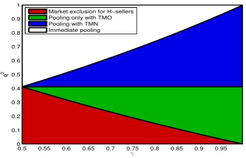
Figure 1.3 illustrates the results of Proposition 1.5.1. Each economy is parametrized by a(γ,q0)coordinate. Depending on time on market observability, different
equilib-ria exist: immediate pooling (white; q0 ≥qIP0 ), pooling with TMN (white and blue; q0≥qS0), pooling with TMO40 (white, blue and green;q0≥qO0), and exclusive market participation by L-sellers irrespective of time on market observability (red;q0<qO0).
Predicting whether H-sellers are more likely to participate in the market when c is “small” or “large” is not clear cut. Naively, lower search costs increase final pay-offs and relax their individual rationality constraint. However, this intuition does not account for how equilibria might change.
On the one hand, if only pooling equilibria existed, a smallercwould enlarge the set of economies in which H-sellers participate in the market; in fact, bothqOc andqNc are
40Forc<c∗the equilibria in Proposition 1.4.3 and 1.4.4 exist for everyq0≥qO
0 andq0≥qN0, respectively. However,
0.5 0.55 0.6 0.65 0.7 0.75 0.8 0.85 0.9 0.95 0
0.1 0.2 0.3 0.4 0.5 0.6 0.7 0.8 0.9 1
γ
q
0
[image:30.595.192.437.90.247.2]Market exclusion for H−sellers Pooling only with TMO Pooling with TMN Immediate pooling
Figure 1.3:Equilibria in different economiesE(γ,q0)forc≤c∗.
decreasing inc. On the other hand, a smallcencourages L-sellers to post high prices and take advantage of buyers’ imperfect signals. Ifq0is belowqOc orqNc H-sellers stay out of the market. Furthermore, pooling prices convey no additional information on the underlying assets, so they rank at the bottom in terms of informational efficiency.
Proposition 1.4.2 characterizes the separating equilibrium and it suggests that a smallcmay reduce trade opportunities when signal precision is sufficiently high. In-deed, for everyq0a separating equilibrium exists only if:
c∈
1−γ
γ (θH−θL),γ(θH−vH)
In a separating equilibrium all sellers participate in the market and trade. Final alloca-tions do not maximize welfare because sellers pay strictly positive search costs, but all sellers eventually trade.
The beneficial signalling effect of search costs may extend to “intermediate” values ofc, i.e. when search costs are too small to create a separating equilibrium but too large to support a pooling equilibrium. Unfortunately, providing a complete equilibrium characterization for all values ofcis a complex endeavor, especially in the TMO case. As a result, I justify this claim through a specific semi-separating equilibrium.
Proposition 1.5.2 Irrespective of time on market observability, there exists a region of parameters(θH,vH,θL,vL,q0,γ)where
• Only L-sellers trade for sufficiently small c.
• For
c∈
γ(1−γ)
γ2+γ−1(vH−θL),
1−γ
γ (θH−θL)
In this semi-separating equilibrium all H-sellers participate in the market and trade. However,γ andcshould be sufficiently high to exclude complete pooling on the same
action. In equilibrium, H-sellers only post a high price and L-sellers mix between the high price andθL. Posted prices do not depend onκ and all sellers trade over time.41
To sum up, search costs can be beneficial by discouraging low quality sellers from pretending to have a high quality good. Although a small c makes participa-tion cheaper, it may worsen adverse selecparticipa-tion, and leave high quality goods out of the market when their initial share is low. In the next section, I consider whether it is pos-sible to enjoy the welfare benefits of low search costs without exacerbating the adverse selection problem.
1.6
Market design
As previously explained, when the costcis small H-sellers may have less incentive to participate in the market. Even when all sellers participate, equilibria are in pooling strategies and prices do not provide any information on product quality. If informa-tional efficiency is considered relevant, this is another loss to take into account.
From a policy perspective, understanding how a benevolent market designer can in-tervene to promote full market participation for the largest possible set of economies is crucial. I adopt a stringent benchmark for the objectives of the market design interven-tion: the resulting equilibrium has to achieve both allocative (see Definition 1.5.1) and informational efficiency (i.e. prices reveal sellers’ types). In my setup, an allocative efficient equilibrium maximizes utilitarian welfare whenc=0.
The market designer is subject to a series of reasonable limitations. First, the mech-anism has to be budget balanced on the equilibrium path. This restriction seems nat-ural as the market should not depend on any external amount of resources to induce participation and trade. Second, transfers cannot be conditional on any posted price. Differently from buyers, the market designer cannot observe currently posted prices. This restriction is consistent with the idea that bilateral transactions involve elements of private negotiation that are difficult to verify externally.42 Therefore, transfers can only be conditional on market participation (τ), trade (r) and, possibly, time on
mar-ket (κ). If time on market is observable, transfers (τκ,rκ) can vary across different
sellers’ cohorts. If instead time on market is not observable, transfers are constant, i.e. (τκ,rκ) = (τ,r). I consider a budget balanced mechanism that satisfies these
41See the proof of Proposition 1.5.2 for a complete characterization of the equilibrium.
42For example, parties may exchange side payments in order to misreport posted prices. Setting up a market
properties to be feasible. For every cohort of sellers, a feasible mechanism has to be ex interim individually rational as a seller knows his type when he participates in the market. I consider a feasible mechanism to beefficient if it leads to an allocative and informationally efficient equilibrium.
Proposition 1.6.1 Let c=0. When time on market is observable an efficient mecha-nism exists only in economies with
q0≥q∗:=max
(
0,1−
γ
1−γ
2
θH−vH
θH−θL )
The efficient market mechanism implements a separating equilibrium with:
• a constant market participation taxτ∗= 1−γγ(θH−θL). • a fixed tax rebate r∗=τ∗
1+1−γ γ q
∗once the seller trades.
For q0<q∗no feasible mechanism improves market outcomes and only L-sellers trade. In equilibrium, a low quality seller postsθL and buyers accept this price for every signal realization, while a high quality seller postsθH and trades once he matches with a buyer who receives a high signal. Prices reveal sellers’ types and the equilibrium is informationally efficient.43 The efficient market intervention is invariant with respect toκbecause transfers do not depend on cohortSκ. This is related to the fact that prices
reveal types, and information on the specific cohort becomes irrelevant for inferring product quality. As(τ∗,r∗)isκ-invariant, the same mechanism is efficient when time
on market is not observable.
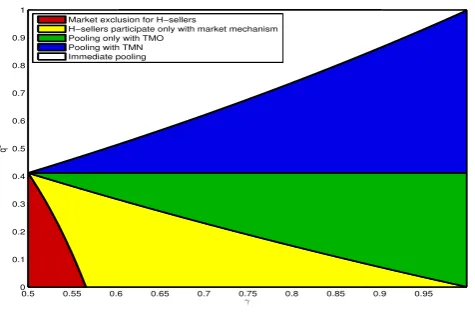
The green and yellow areas in Figure 1.4 illustrate the improvement due to(τ∗,r∗).
Without a market intervention, an equilibrium is allocative efficient only if q0≥qS0 (blue and white areas). When time on market is observable, H-sellers could also par-ticipate in the market in economies in the green areaq0∈[qO0,qS0), but they would not trade for sure. No high quality seller participates in economies in the yellow and red areas.
Proposition 1.6.1 points out that the mechanism(τ∗,r∗)may support an allocative
and informational efficient allocation for everyq0∈(0,1)only if:
γ ≥
√
θH−θL √
θH−θL+ √
θH−vH :=γ∗
43In supplementary work, I relax the requirement of informationally efficient prices and explore whether it is possible
0.5 0.55 0.6 0.65 0.7 0.75 0.8 0.85 0.9 0.95 0
0.1 0.2 0.3 0.4 0.5 0.6 0.7 0.8 0.9 1
γ
q
0
Market exclusion for H−sellers
H−sellers participate only with market mechanism Pooling only with TMO
[image:33.595.200.438.90.250.2]Pooling with TMN Immediate pooling
Figure 1.4:Efficient market intervention(τ∗,r∗).
Despite the improvement, it is still not possible to implement a first best allocation in every economy. Ifγ<γ∗an efficient allocation is possible only ifq0≥q∗>0 (see the
red area in Figure 1.4).44 Otherwise, it is not possible to mitigate adverse selection with a feasible market intervention. In these economies, the mechanism(τ∗,r∗)violates the
individual rationality constraint of H-sellers because of the budget balance restriction. High and low quality sellers have different expected time on market (1
γ and 1 periods
respectively), and budget balance leads to an implicit transfer from high to low quality sellers, reducing the former’s expected payoff. A high quality seller prefers to stay out of the market when this expected transfer outweighs his gains from trade.
1.7
Conclusion
Several theoretical papers point out the existence of an ITS equilibrium in markets with asymmetric information on asset quality. All sellers participate in the market: low quality sellers trade early, and high quality sellers trade later at higher prices. Since most markets offer multiple opportunities to sell, these results seem favorable