Data driven approach to machine condition prognosis using least square regression trees

Data-driven approach to machine condition prognosis

using least square regression trees

Van Tung Tran, Bo-Suk Yang*

Abstract

Machine fault prognosis techniques have been profoundly considered in the recent time due to their substantial profit for reducing unexpected faults or unscheduled maintenance. With those techniques, the working conditions of components, the trending of fault propagation, and the time-to-failure are precisely forecasted before they reach the failure thresholds. In this work, we propose an approach of Least Square Regression Tree (LSRT), which is an extension of the Classification and Regression Tree (CART), in association with one-step ahead prediction of time-series forecasting techniques to predict the future condition of machine. In this technique, the number of available observations is firstly determined by using Cao’s method and LSRT is employed as prediction model in the next step. The proposed approach is evaluated by real data of low methane compressor. Furthermore, a comparison of the predicted results obtained from CART and LSRT are carried out to prove the accuracy. The predicted results show that LSRT offers a potential for machine condition prognosis.

Keywords: Least square method; Embedding dimension; Regression trees; Prognosis; Time-series forecasting

1. Introduction

Failure prediction, which is addressed in this paper, allows pending failures to be early identified before they come to be more serious failures that result in machine breakdown and repair costs. RUL is the time left for the normal operation of machine before the breakdown occurs or machine condition reaches the critical failure threshold. However, prognosis is a relatively new area and becomes a significant part of CBM [2]. Various approaches in prognosis which range in fidelity from simple historical failure rate models to high-fidelity physics-based models have been developed. Fig. 1 illustrates the hierarchy of potential prognostic approaches related to their applicability and relative accuracy as well as their complexity. Each of them has advantages and limitations in application. For example, experience-based prognosis is the least complex, however, it is only utilized in situations where the prognostic model is not warranted due to low failure occurrence rate; trend-based prognosis may be implemented on the subsystems with slow degradation type faults [3].

Fig. 1 Fidelity of prognostic approaches

In these approaches, data-driven based and model-based are the most considered because they provide higher accuracy and reliability. Nevertheless, model-based techniques require accurate mathematical models of failure modes and are merely applied in some specific components in which each of them needs different model. Furthermore, a suitable mathematical model is also difficult to establish and changes in structural dynamics can affect the mathematical model which is impossible to mimic the behavior of systems. Meanwhile, data-driven techniques utilize and require a large amount of historical data to build a prognostic model. Most of these techniques use artificial intelligence which can generate the flexible and appropriate models for almost failure modes. Consequently, data-driven approaches that some of those have been proposed in references [4-7] are firstly examined.

value and not too large to avoid the unnecessary increase in computational complexity. False nearest neighbor method (FNN) [8] and Cao’s method [9] are commonly used to determine this value. However, FNN method not only depends on chosen parameters and the number of available observations but also is sensitive to additional noise. Cao’s method overcomes the shortcomings of the FNN approach and therefore, it is chosen in this study.

Classification and regression trees (CART) [10] handle multivariate regression methods to obtain models. These models have proven to be quite interpretable and competitive predictive accuracy. Moreover, these models can be obtained through a computational efficiency that hardly has parallel in competitive approaches, turning these models into a good choice for a large variety of data mining problems where these features play a major role [11]. CART is widely implemented in machine fault diagnosis. In the prediction techniques, CART is also applied to forecast the short-term load of the power system [12] and predict the future conditions of machines [13]. Nevertheless, the average value of samples in each terminal node used as predicted result is the reason for reducing the accuracy of CART. Several approaches have been proposed to ameliorate that CART’s limitation [14-16]. In this paper, least square method [17] to improve the prediction capability of CART model is proposed. This improved model is then used to predict the conditions of machine.

2. Background knowledge

2.1. Determine the embedding dimension

Assuming a time-series of x1, x2, …, xN. The time delay vector is defined as follows [13]:

τ

τ,..., ], 1,2,..., ( 1)

,

[ ( 1)

)

( = x x+ x+ − i= N− d−

y_{id i i i d} (1)

where τ is the time delay and d is the embedding dimension. Defining the quantity as follows:

) ( ) ( ) 1 ( ) 1 ( ) , ( ) , ( ) , ( d y d y d y d y d i a d i n i d i n i − + − + = (2)

where ||⋅|| is the Euclidian distance and is given by the maximum norm, yi(d) means the ith reconstructed vector and n(i, d) is an integer so that yn(i,d)(d) is the nearest neighbor of yi(d) in the embedding dimension d.

¦

E(d) is only dependent on the dimension d and the time delay τ. To investigate its variation from d to d+1, the parameter E1 is given by

) ( ) 1 ( ) ( 1 d E d E d

E = + (4)

By increasing the value of d, the value E1(d) is also increased and it stops increasing when

the time series comes to a deterministic process. If a plateau is observed for d • d0 then d0 + 1 is

the minimum embedding dimension.

The Cao’s method also introduced another quantity E2(d) to overcome the problem in

practical computations where E1(d) is slowly increasing or has stopped changing if d is large

enough: ) ( ) 1 ( ) ( 2 d E d E d E _∗ ∗ + = (5) where

¦

According to [8], for purely random process, E2(d) is independent of d and equal to 1 for any

of d. However, for deterministic time-series, E2(d) is related to d. Consequently, there must exist

some d’s so that E2(d)  1.

2.2. Least square regression trees (LSRT)

A regression tree models are sometimes called piecewise constant regression models. Regression trees are constructed using a recursive partitioning algorithm. Assuming that a learning set comprised n couples of observation(y1,x1),...,(yn,xn), where xi =(x1_i,...,xd_i)is a set

of independent variables and y_i∈R is a response associated with xi. The regression tree is constructed by using recursively partitioning process of this learning set into two descendant subsets which are as homogeneous as possible until the terminal nodes are achieved.

The split values for partitioning process are chosen so that the sums of square errors are minimized. The sum of square error of the tth subset is expressed as:

( )

(

)

, 1 ( ) i i i y t

R t y y t

n ∈

=

¦

x

(7)

respectively. At each terminal node, the predicted response is estimated by the average y t( )of all values y of the response variables associated to that node. This issue is the reason why the prediction accuracy is significantly reduced.

To improve the accuracy of predicted response, the mean value ( )y t of response at any node in LSRT is replaced by the local modelf(ș,xi), which shows the relationship between the

response yi and a set of independent variable xi. Hence, the sum of square error of the tth node (subset) in Eq. (7) can be rewritten as:

(

)

, 1 ( ) ( , ) i i i i y t

R t y f

n ∈

=

¦

x

ș _{x (8)}

where θθθθ is a set of parameters. The local modelsf(ș,xi) can be either linear or non-linear

model in which the forms are known with unknown values of parameters as shown in Table 1.

Table 1 Local model types in LSRT

In LSRT, those local models are organized as a set of models. At any node, an appropriate model f(ș,xi)is chosen to fit the independent variable xi. The values of parameters θθθθ of each model are initially calculated by using least square method [17]:

1

[ T ] Ty

θ −

= X X X (9)

where y=[ ,...,y₁ y_n]Tis the response , X=[x₁T,...,xT T_n] is a matrix of independent variables. Furthermore, there could be several appropriate local models that are found, the best model are subsequently chosen based on the minimum of the sum of squares due to error (SSE) and the root mean squared error (RMSE) criterions:

¦

¦

where yi andyˆi are response value and predicted value given by local model at that node,

respectively. By this improvement, the outputs of terminal nodes are local models that lead to more accurate prediction.

Similarly to CART, LSRT needs to be pruned and carried out cross-validation in order to avoid the over-fitting and complicated problems. These processes are implemented as in references [13].

3. Proposed system

vibration data, the proposed system as shown in Fig. 2 is proposed. This system consists of four procedures sequentially: data acquisition, data splitting, training-validating model and predicting. The role of each procedure is explained as follows:

Fig. 2 Proposed system for machine fault prognosis

Step 1 Data acquisition: acquiring vibration signal during the running process of the machine until faults occur.

Step 2 Data splitting: the trending data is split into two parts: training data for building the model and testing data for testing the validated model.

Step 3 Training-validating: determining the embedding dimension based on Cao’s method, building the model and validating the model for measuring the performance capability.

Step 4 Predicting: one-step-ahead prediction is used to forecast the future value. The predicted result is measured by the error between predicted value and actual value in the testing data. If the prediction is successful, the result obtained from this procedure is the prognosis system.

4. Experiments and results

The proposed method is applied to real system to predict the trending data of a low methane compressor of a petrochemical plant. This compressor shown in Fig. 3 and is driven by a 440 kW motor, 6600 volt, 2 poles and operating at a speed of 3565 rpm. Other information of the system is summarized in Table 2.

Fig. 3 Low methane compressor Table 2 Description of system

The condition monitoring system of this compressor consists of two types, namely off-line and on-line. In the off-line system, accelerometers were installed along axial, vertical, and horizontal directions at various locations of drive-end motor, non drive-end motor, male rotor compressor and suction part of compressor. In the on-line system, accelerometers were located at the same positions as in the off-line system but only in the horizontal direction.

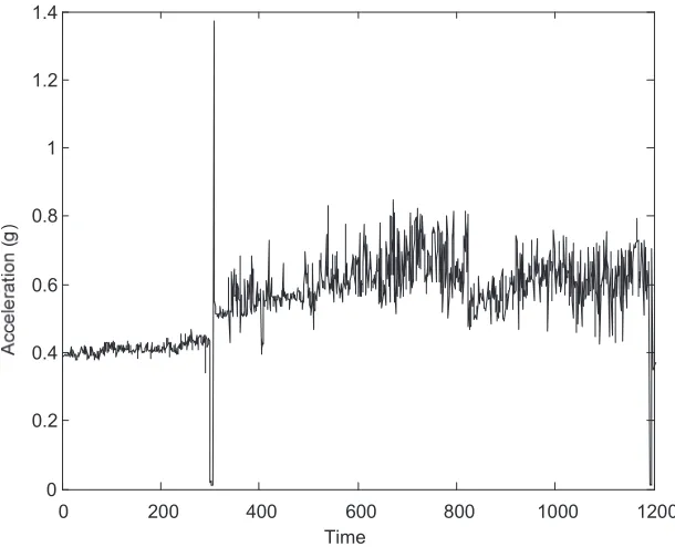
Fig. 4 The entire of peak acceleration data of low methane compressor Fig. 5 The entire of envelope acceleration data of low methane compressor

These figures show that the machine was in normal condition during the first 300 points of the time sequence. After that time, the condition of the machine suddenly changed. This indicates possible faults occurring in the machine. By disassembling and inspecting, these faults were identified as the damage of main bearings of the compressor (notation Thrust: 7321 BDB) due to insufficient lubrication. Consequently, the surfaces of these bearings were overheated and delaminated [13].

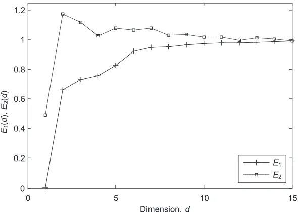
With the aim of forecasting the change of machine condition, the first 300 points are used to train the system. Before being used to generate the prediction models, the time delay and the embedding dimension are initially determined. The time delay is chosen as 1 for the reason that one step-ahead is implemented in all datasets, whilst the embedding dimension is calculated according to the method mentioned in section 2.1. Theoretically, the minimum embedding dimension is chosen as E1(d) obtains a plateau. In Fig.6, the embedding dimension is chosen as

6 for the reason that the values of E1(d) reaches its saturation.

Fig. 6 The values of E

1 and E2 of peak acceleration data of low methane compressor

Subsequent to determining the time delay and embedding dimension, the process of generating the prediction model is carried out. It is noted that during the process of building the prediction model (regression tree model), the number of response values for each terminal node in tree growing process is 5 and the number of cross-validations is chosen as 10 to select the best tree in tree pruning. Furthermore, in order to evaluate the predicting performance, the RMSE value given in Eq. (10) is utilized. Fig. 7 depicts the training and validating results of LSRT for peak acceleration data. The actual values and predicted values are almost identical with very small RMSE of 0.00118. It indicates that the learning capability of LSRT model is tremendously positive.

Fig. 7 Training and validating results of peak acceleration data

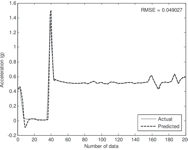
for peak acceleration data with the small RMSE error of 0.049. Moreover, it can closely track with the changes of the operating condition of machine that is impossible to be obtain with CART as shown in Fig. 9. This is of crucial importance in industrial application for pending failures of equipments.

Fig. 8 Predicted results of peak acceleration data using LSRT Fig. 9 Predicted results of peak acceleration data using CART

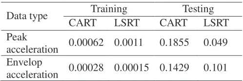
Table 3 shows the remaining results of applying LSRT on envelop acceleration data. It is also depicts the comparison of the RSME between CART and LSRT. According to Table 3, training results of CART are sometimes slightly smaller than those of LSRT but the testing results of CART are always larger. This indicates the superiority of LSRT in aspect of machine condition prognosis.

Table 3 The RMSE of CART and LSRT

5. Conclusions

Machine condition prognosis is extremely significant in foretelling the degradation of working condition and trends of fault propagation before they reach the alarm. In this study, the machine prognosis system based on one-step-ahead of time-series techniques and least square regression trees has been investigated. The proposed method is validated by predicting future state conditions of a low methane compressor wherein the peak acceleration and envelope acceleration have been examined. The predicted results of the LSRT are also compared with those of traditional CART. From the predicted results, the LSRT model performance is vastly superior to the traditional model, especially in testing process. Additionally, the predicted results of LSRT are capable of tracking the change of machines’ operating conditions with high accuracy. The tracking-change capability of operating conditions is of crucial importance in pending failures of industrial equipments. The results confirm that the proposed method offers a potential for machine condition prognosis with one-step-ahead prediction.

References

[1]. Byington, C.S., Watson, M., Roemer, M.J., Galic, T.R, McGroarty, J.J. (2003). Prognostic

enhancements to gas turbine diagnostic systems, Proceeding of IEEE Aerospace Conference, 7

[2]. J. Luo, M. Namburu, K. Pattipati, L. Qiao, M. Kawamoto and S. Chigusa, Model-based

prognostic techniques, Proceedings of IEEE Systems Readiness Technology Conference, (2003)

330-340.

[3]. M. J. Roemer, C. S. Byington, G. J. Kacprzynski and G. Vachtsevanos, An overview of

selected prognostic technologies with application to engine health management, Proceedings of

ASME GT2006-90677, (2006).

[4]. G. Vachtsevanos and P. Wang, Fault prognosis using dynamic wavelet neural networks,

Proceedings of IEEE Systems Readiness Technology Conference, (2001) 857-870.

[5]. R. Huang, L. Xi, X. Li, C. R. Liu, H. Qiu and J. Lee, Residual life prediction for ball bearings

based on self-organizing map and back propagation neural network methods, Mechanical

Systems and Signal Processing, 21 (2007) 193–207.

[6]. W.Q. Wang, M.F. Golnaraghi and F. Ismail, Prognosis of machine health condition using

neuro-fuzzy system, Mechanical System and Signal Processing, 18 (2004) 813-831.

[7]. W. Wang, An adaptive predictor for dynamic system forecasting, Mechanical Systems and

Signal Processing, 21 (2007) 809–823.

[8]. M.B. Kennel, R. Brown and H.D.I. Abarbanel, Determining embedding dimension for

phase-space reconstruction using a geometrical construction, Physical Review A, 45 (1992) 3403–

3411.

[9]. L. Cao, Practical method for determining the minimum embedding dimension of a scalar time

series, Physica D, 110 (1997) 43–50.

[10].L. Breiman, J.H. Friedman, R.A. Olshen and C.J. Stone, Classification and regression trees,

Chapman & Hall (1984).

[11]. L. Torgo, A study on end-cut preference in least squares regression trees, University of Porto,

http://www.liacc. up.pt/~ltorgo (2008).

[12].J. Yang and J. Stenzel, Short-term load forecasting with increment regression tree, Electric

Power Systems Research, 76 (2006) 880-888.

[13].V.T. Tran, B.S. Yang, M.S. Oh and A.C.C. Tan, Machine condition prognosis based on

regression trees and one-step-ahead prediction, Mechanical Systems and Signal Processing, 22

(2008) 1179-1193.

[14].A. Suárez and J.F. Lutsko, Globally optimal fuzzy decision trees for classification and

regression, IEEE Trans. on Pattern Analysis and Machine Intelligence, 21 (1999) 1297-1311.

[15].C. Huang and J.R.G. Townshend, A stepwise regression tree for nonlinear approximation:

application to estimating subpixel land cover, International Journal of Remote Sensing, 24

(2003) 75-90.

[16].D.S. Vogel, O. Asparouhov and T. Scheffer, Scalable look-ahead linear regression trees,

Proceedings of the 13th International Conference on Knowledge Discovery and Data Mining

(2007) 757-764.

3 UR

J Q R

V WLF

D S S

UR D F_K

Fig. 1 Fidelity of prognostic approaches

!

!" _"

#

$%&$% $%&$%

$%&$%"

'

Fig. 3 Low methane compressor

( ) * + (

,( ,) ,* ,+ ,( ,)

.

Fig. 5 The entire envelope acceleration data of low methane compressor

/ /

,( ,) ,* ,+ ,(

$, G

(

G

,

((

G

( (₍

0 50 100 150 200 250 300 0.34

0.36 0.38 0.4 0.42 0.44 0.46

Number of data

A

c

c

e

le

ra

ti

o

n

(

g

)

RMSE = 0.0011883

Actual Predicted

Fig. 7 Training and validating results of peak acceleration data.

0 20 40 60 80 100 120 140 160 180 200 -0.2

0 0.2 0.4 0.6 0.8 1 1.2 1.4 1.6

Number of data

A

c

c

e

le

ra

ti

o

n

(

g

)

RMSE = 0.049027

Actual Predicted

/ / ,( ,) ,* ,+ ,( ,) -. 0

Fig. 9 Predicted results of peak acceleration data using CART.

Table 1 Local model types in LSRT

Model type Description Parameters Polynomial

¦

+ = − + = 1 1 1 n i i n ix

y θ θ_i

Power 3 2 2 1 1 θ θ θ θ θ x y x y + = = 3 2 1,θ ,θ

θ Fourier

¦

¦

0,θ ,θ

θ

Sine

¦

=

+ =

n

i i i i

x y

1

3 2

1 sin(θ θ )

θ θ1_i,θ2_i,θ3_i

Table 1 Description of system

Electric motor Compressor

Voltage 6600 V Type Wet screw

Power 440 kW

Lobe Male rotor (4 lobes)

Pole 2 Pole Female rotor (6 lobes)

Bearing NDE:#6216, DE:#6216

Bearing Thrust: 7321 BDB

Table 3 The RMSE of CART and LSRT

Data type Training Testing

CART LSRT CART LSRT

Peak

acceleration 0.00062 0.0011 0.1855 0.049 Envelop