Robust Asset Allocation Under
Model Ambiguity
Sandrine Tobelem - Foldvari
Department of Statistics
The London School of Economics and Political Sciences
A thesis submitted for the degree of
Doctor of Philosophy
I certify that the thesis I have presented for examination for the MPhil/PhD
degree at the London School of Economics and Political Science is solely my own
work other than where I have clearly indicated that it is the work of others (in
which case the extent of any work carried out jointly by me and any other person is clearly identified in it).
The copyright of this thesis rests with the author. Quotation from it is permitted,
provided that full acknowledgement is made. This thesis may not be reproduced
without the prior written consent of the author.
I warrant that this authorisation does not, to the best of my belief, infringe the
Acknowledgements
Starting a PhD is like embarking upon a very long and uncertain journey. Support is a key component for success, and I am extremely
grateful I have been helped so much throughout the long six years I
spent writing this thesis.
I would like to thank the Statistics Department at the London School
of Economics and Political Sciences that allowed me to undertake
an especially difficult part-time PhD. I would like to acknowledge in
particular the academic help I received from Pr Ragnar Norberg, Pr
Qiwei Yao, Pr Umut Cetin and Pr Henry Wynn. I also would like to thank the administrative staff of the department and in particular
Ian Marshall. Thank to my fellow LSE PhD students; even if I did
not meet with them often, they still made me feel I was part of the
research department.
I would like to acknowledge the financial support of the CREST in
Paris for the grant I received for the first two years of my PhD, and
especially Pr Christian Gourieroux, Pr Laurence Lescourret and Pr
Nizar Touzi.
I also would like to thank my current employer Credit Suisse, which
financed the remaining four years of my research, and gave me enough
flexibility in my job to be able to complete my thesis, despite a very
challenging and demanding environment. I particularly would like to
I especially would like to thank Yves Bentz, my previous manager
at Credit Suisse, who initially offered me to work at the bank while
completing my PhD. He has been a real inspiration and support in
all respects.
I also would like to acknowledge the help and advice I received from
Pr Monique Jean-Blanc, Pr Bernard Sinclair-Desgagne and especially Pr Leonard Smith and Pr Rudiger Kiesel.
I thank all my friends, and especially David Le Bris and Judith
Byd-lowski who devoted time reading parts of my PhD and giving me
sensible and most welcome advice.
But first and foremost, I would like to thank my PhD supervisor, Pr
Pauline Barrieu. I will never be able to express enough gratitude. She
has been incredibly inspiring, guiding me through every step, never
letting me give up and encouraging me in my most difficult times.
She became a very dear and important person to me and I owe her
much more than the great achievement of finishing my PhD thesis.
I thank warmly my family, my parents and my brother and my parents
in law who gave me confidence and emotional support.
Finally, I would like to thank my husband Peter. He supported me
the most completely and always believed I would finish my PhD thesis
even when I was convinced I could never do it. He gave me an infinite
supply of time, trust and love and I would like to dedicate my research to him, as I could not have done it without his unconditional support.
I also dedicate my PhD thesis to our two lovely baby daughters Laura
Abstract
A decision maker, when facing a decision problem, often considers several models to represent the outcomes of the decision variable
con-sidered. More often than not, the decision maker does not trust fully
any of those models and hence displays ambiguity or model
uncer-tainty aversion.
In this PhD thesis, focus is given to the specific case of asset allocation
problem under ambiguity faced by financial investors. The aim is not
to find an optimal solution for the investor, but rather come up with
a general methodology that can be applied in particular to the asset allocation problem and allows the investor to find a tractable, easy to
compute solution for this problem, taking into account ambiguity.
This PhD thesis is structured as follows: First, some classical and
widely used models to represent asset returns are presented. It is
shown that the performance of the asset portfolios built using those
single models is very volatile. No model performs better than the
others consistently over the period considered, which gives empirical
evidence that: no model can be fully trusted over the long run and that several models are needed to achieve the best asset allocation
possible. Therefore, the classical portfolio theory must be adapted
to take into account ambiguity or model uncertainty. Many authors
have in an early stage attempted to include ambiguity aversion in
the asset allocation problem. A review of the literature is studied
lack flexibility and tractability. The search for an optimal solution
to the asset allocation problem when considering ambiguity aversion
is often difficult to apply in practice on large dimension problems,
as the ones faced by modern financial investors. This constitutes the motivation to put forward a novel methodology easily applicable,
robust, flexible and tractable. The Ambiguity Robust Adjustment
(ARA) methodology is theoretically presented and then tested on a
large empirical data set. Several forms of the ARA are considered and
tested. Empirical evidence demonstrates that the ARA methodology
improves portfolio performances greatly.
Through the specific illustration of the asset allocation problem in
finance, this PhD thesis proposes a new general methodology that will hopefully help decision makers to solve numerous different problems
Contents
1 Introduction 1
2 Classical Approaches to the Asset Allocation Problem 7
2.1 Framework . . . 9
2.1.1 Notation and setting . . . 10
2.1.2 Trading Strategy . . . 12
2.1.3 Decision under risk . . . 13
2.1.4 The classical portfolio optimisation problem . . . 13
2.2 The Efficient Frontier, Markowitz (1952) . . . 14
2.2.1 Background . . . 15
2.2.1.1 The mean-variance paradigm . . . 15
2.2.1.2 The concept of diversification . . . 16
2.2.1.3 Efficient Frontier Definition . . . 17
2.2.2 The Efficient Frontier without a risk-free asset . . . 18
2.2.2.1 The Minimum Variance portfolio . . . 19
2.2.2.2 The Maximum Sharpe ratio portfolio . . . 19
2.2.2.3 The Two Fund Theorem. . . 21
2.2.3 Introduction of a risk-free asset . . . 22
2.2.3.1 Tangential portfolio . . . 23
2.2.3.2 The One Fund Theorem. . . 24
2.3 The Capital Asset Pricing Model (CAPM), Sharpe (1964) . . . . 25
2.3.1 The Capital Market Line (CML) . . . 26
2.3.1.1 The Market Portfolio . . . 26
2.3.1.2 The CML Equation . . . 28
CONTENTS
2.3.2.1 The CAPM Betas . . . 28
2.3.2.2 The SML Equation . . . 29
2.3.3 The CAPM . . . 30
2.3.3.1 The CAPM Equation . . . 30
2.3.3.2 The Jensen Alpha . . . 31
2.4 The Asset Pricing Theory (APT), Ross(1976) . . . 33
2.4.1 The APT Framework . . . 34
2.4.2 APT Theorem . . . 35
2.4.3 Construction of a factor model portfolio . . . 37
2.5 Performance measures . . . 38
2.6 Appendix . . . 41
2.6.1 Efficient Frontier without a risk-free asset . . . 41
2.6.2 Efficient Frontier with a risk-free asset . . . 43
3 Factor Model Performances: Empirical Evidence 46 3.1 General remarks on factor models . . . 48
3.1.1 Factor models objectives . . . 48
3.1.2 Types of factor models . . . 49
3.2 Presentation of the data . . . 51
3.2.1 The raw data . . . 51
3.2.2 The cleaning process . . . 53
3.2.3 The returns . . . 54
3.2.3.1 Computation and cleaning process . . . 54
3.2.3.2 Some basic statistics . . . 55
3.3 The Capital Asset Pricing Model (CAPM) . . . 58
3.3.1 Estimation of the CAPM model . . . 58
3.3.1.1 Betas Estimation . . . 58
3.3.1.2 Goodness of fit of the CAPM . . . 59
3.3.2 Betas instability . . . 60
3.3.2.1 Betas time series . . . 61
3.3.2.2 Stationary tests . . . 62
3.3.3 The Jensen statistics . . . 64
CONTENTS
3.4.1 The exogenous factors . . . 67
3.4.1.1 Expected sensitivities toward the exogenous factors 67 3.4.1.2 Exogenous factor returns and index returns . . . 68
3.4.2 The EFM model . . . 71
3.4.3 Results . . . 72
3.4.3.1 Betas instability . . . 72
3.4.3.2 Jensen statistics . . . 73
3.5 A Fundamental Factor Model (FFM) . . . 75
3.5.1 The FFM model . . . 75
3.5.1.1 The FFM factors . . . 75
3.5.1.2 FFM equation . . . 76
3.5.2 Estimation of the FFM model . . . 76
3.5.3 Comments on the FFM . . . 78
3.6 Principal Component Analysis (PCA) . . . 79
3.6.1 The PCA model . . . 79
3.6.1.1 The PCA principle . . . 79
3.6.1.2 Factors selection and Betas calibration . . . 80
3.6.2 PCA Estimation and Results . . . 81
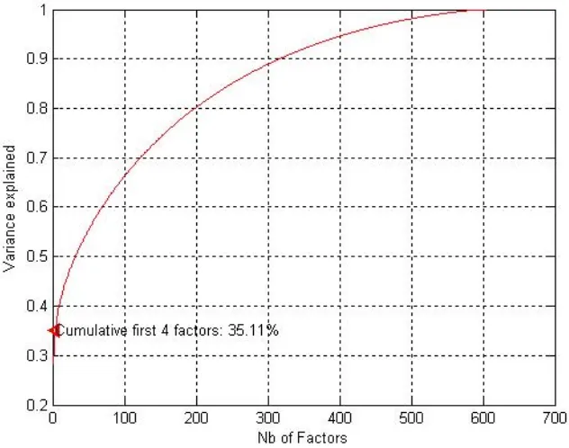
3.6.2.1 Explanatory power of the PCA . . . 81
3.6.2.2 PCA Factors Identification . . . 82
3.6.2.3 The Jensen Statistics . . . 84
3.6.3 Comment on the PCA model . . . 85
3.7 Independent Component Analysis (ICA) . . . 86
3.7.1 ICA principle . . . 86
3.7.2 ICA Fast Algorithm . . . 87
3.7.2.1 Negentropy: a measure of non-Gaussianity . . . . 88
3.7.2.2 Mutual information . . . 88
3.7.3 Estimation of the model . . . 89
3.8 Clusters Analysis (CA) . . . 91
3.8.1 Cluster Analysis principle . . . 92
3.8.2 Methodology . . . 92
3.8.3 Estimation of the model . . . 94
CONTENTS
4 Decision Under Ambiguity: Literature Review 99
4.1 The concept of Ambiguity . . . 100
4.1.1 The Knight Uncertainty . . . 100
4.1.2 Savage Subjective Expected Utility (1954) . . . 101
4.1.3 The Ellsberg Paradox . . . 102
4.1.4 Kahneman and Tversky Prospect Theory (1979) . . . 105
4.2 Decision under Ambiguity . . . 106
4.2.1 Gilboa and Schmeidler Max-Min Expected Utility (1989) . 106 4.2.2 Hansen and Sargent Robust Control (2001) . . . 107
4.3 Portfolio Allocation and Model Risk . . . 108
4.3.1 The classical Markowitz settings . . . 109
4.3.2 Learning and Filtering . . . 110
4.3.2.1 Classical Learning: the Bayesian approach . . . . 110
4.3.2.2 Learning Under Ambiguity . . . 113
4.3.2.3 The shrinkage approach . . . 115
4.3.2.4 The Multiple Prior Approach . . . 115
4.3.3 Generalised framework to model ambiguity in the asset al-location problem . . . 116
4.3.3.1 A smooth class of preferences that models ambiguity117 4.3.3.2 A Generalised Model . . . 117
4.4 The Poor Performance of Ambiguity Models on Empirical Data. . 118
5 A Robust Alternative Approach to Model Ambiguity 121 5.1 Settings . . . 123
5.2 An alternative robust approach to model uncertainty: the Ambi-guity Robust Adjustment (ARA) . . . 125
5.2.1 The Absolute Ambiguity Robust Adjustment (AARA) . . 127
5.2.2 The Relative Ambiguity Robust Adjustment (RARA) . . . 131
5.2.3 The role of the risk free asset . . . 132
5.2.4 ARA parameterisation . . . 133
5.3 Some definitions relative to the ARA asset allocation . . . 134
CONTENTS
5.4.2 Results . . . 138
5.5 A parametrized model application . . . 140
5.5.1 Settings . . . 141
5.5.2 The ARA transformation . . . 142
5.5.3 Asymptotic behaviour of the ARA weights . . . 145
5.5.3.1 ARA weights asymptotic behaviour when γ → ∞ 145 5.5.3.2 ARA weights asymptotic behaviour when γ →0 . 146 5.5.3.3 ARA weights for different values of the parameter γ146 5.6 Conclusion . . . 146
5.7 Appendix . . . 149
5.7.1 ARA-KMM weights comparison . . . 149
5.7.1.1 Computation of the ARA weights . . . 149
5.7.1.2 ARA and KMM weights comparison . . . 151
5.7.2 Theoretical illustration . . . 152
5.7.2.1 Computation of φARA . . . . 152
5.7.2.2 Computation of φARA,1(0) . . . . 152
5.7.2.3 Computation of φARA,2(0) . . . . 153
6 Evidence from Empirical Study : Outperformance of the ARA Portfolio 154 6.1 Empirical study framework . . . 155
6.1.1 Dataset and notations . . . 156
6.1.2 Portfolios tested . . . 156
6.1.2.1 Single strategies considered . . . 157
6.1.2.2 Combined portfolios . . . 159
6.1.3 Performance measures . . . 161
6.2 Calibration and empirical portfolio performances . . . 163
6.2.1 Single portfolios performances . . . 163
6.2.2 Calibration of the absolute ambiguity parameter γ and the relative ambiguity adjustment π . . . 167
6.2.3 The SEU portfolio performance . . . 170
6.2.4 The ARA portfolio performance . . . 174
CONTENTS
6.4 Appendix: Estimation of the empirical inverse of the covariance
matrix . . . 178
7 Nonlinear Relative Ambiguity Adjustment 179 7.1 A nonlinear, non-parametric method to estimate π: the Support Vector Machines (SVM) . . . 181
7.1.1 The SVM theory . . . 181
7.1.1.1 Basic theory: linear SVM . . . 182
7.1.1.2 Nonlinear SVM . . . 183
7.1.2 Empirical application: nonlinear ARA portfolio calibrated with the SVM algorithm . . . 184
7.1.2.1 Framework and calibration of the SVM algorithm 184 7.1.2.2 Comparison of the SVM generated ARA portfo-lio performance against the SEU and linear ARA portfolio performances . . . 187
7.1.2.3 Main drawbacks of the SVM algorithm to cali-brate π. . . 188
7.2 A more ad hoc method to calibrate a nonlinear form for π . . . . 188
7.2.1 Some nonlinear desired properties of the Relative Ambigu-ity Robust Adjustment π . . . 189
7.2.1.1 Weight dispersion across the different models . . 189
7.2.1.2 Precautionary principle . . . 190
7.2.1.3 The global ambiguity aversion . . . 190
7.2.2 Ad hoc nonlinear form for π for the ARA allocation . . . . 191
7.2.2.1 Prior specification of the function π . . . 192
7.2.2.2 Results and Comments . . . 193
7.3 Conclusion . . . 194
8 Conclusion 197
List of Figures
2.1 Efficient Frontier . . . 23
2.2 Efficient Frontier with a risk-free asset . . . 25
2.3 Security Market Line . . . 32
3.1 Cumulative Indexes Returns in % . . . 55
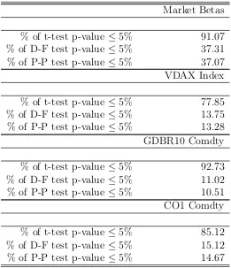
3.2 Market Betas . . . 59
3.3 CAPM R2 . . . . 60
3.4 CAPM Residuals QQ Plot . . . 61
3.5 Exogenous Cumulative Factors Returns in % . . . 69
3.6 Fundamental Factors Returns / Stocks Returns Correlation in % . 77 3.7 PCA Factor Cumulative Explanatory Power . . . 82
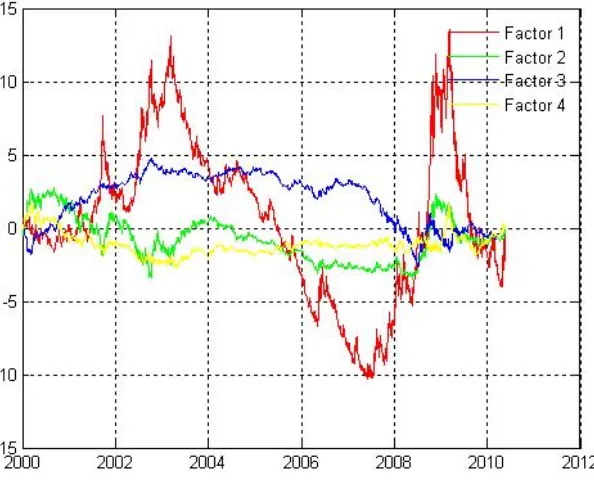
3.8 PCA First 4 Factors Returns . . . 83
3.9 Mean Alpha vs. Number of PCA factors selected . . . 86
3.10 ICA First 4 Factors Returns . . . 90
3.11 ICA Alphas vs. Number of Independent Components . . . 92
3.12 Factor Models Cumulative Returns (%) . . . 98
5.1 ψ for different values of the ambiguity aversion parameter γ . . . 130
5.2 KMM weights . . . 139
5.3 ARA weights . . . 139
5.4 φARA . . . . 147
6.1 Strategies Returns without transaction costs . . . 165
6.2 Strategies Returns with 3 basis points transaction costs . . . 165
6.3 Performance measures . . . 168
LIST OF FIGURES
6.5 Ambiguity Robust Adjusted Strategies Returns . . . 174
7.1 SEU, ARA and SVM strategies Hit ratios . . . 187
Chapter 1
Introduction
”Success is not final, failure is not fatal: it is the courage to continue that counts.”
Sir Winston Churchill.
A decision-maker, when facing a decision problem, often considers several models
in order to represent the possible outcomes of the decision variables considered.
More often than not, the decision-maker does not fully trust any of the models
considered, and, hence, displays ambiguity, or model uncertainty aversion. In this
PhD thesis, the generic terminology ’model uncertainty’, or ’ambiguity’ is used
to refer to any situation where a decision-maker has to consider different models,
different scenarii, or, has to rely on different experts (that may all be wrong, or at least subject to error), to come to a decision. The general term ’prior’
de-scribes a model, scenario, or expert’s opinion. The question of how ambiguity
aversion should be taken into account in the decision-making problem has,
there-fore, arisen, and has now become crucial in many scientific fields (including but
not limited to: economics, biology, physics, climatology and finance).
There is a substantial body of literature on the problem of decision-making under
ambiguity. The classical approaches have significant limitations: they often prove
limitations, a methodology to operate a trade-off between robustness and
opti-misation has been proposed. Since the complexity of most practical frameworks
makes this task almost impossible with current limitations, the objective has not
been to find the ”optimal” decision for the decision-maker; the focus has been, rather, on a robust approach that allows the decision-maker to combine different
priors in a practical and tractable way - and to take the best decision - in a robust
sense (i.e. that can be easily adapted to the different types and number of priors
considered). The question is, really, about finding a solution that encompasses all
the different information given by the different priors, but also the ambiguity the
decision-maker faces regarding the set of priors; in other words, finding a robust
decision rule, as defined by Levin & Williams (2003): a rule that ”although not
exactly optimal for any prior, yields outcomes that are acceptable to all priors”.
The contribution of this PhD thesis is therefore to provide the decision maker
with a novel methodology that deals with model ambiguity in an original fashion.
In this thesis, focus is given to the financial field to illustrate decision-making
under ambiguity. The novel methodology proposed in this PhD theisi is applied
to the asset allocation problem of an investor, when ambiguous about the models
used to describe the asset returns distribution, providing a practical, systematic
algorithm to trade a large portfolio of assets.
The Modern Portfolio Theory, initiated with the classical Markowitz framework,
aims at solving the asset allocation problem. Many authors have, since then,
considered more complex settings, allowing the investor to take into account sev-eral models for risky asset return distributions. Indeed, many different models
can be used in finance to represent asset returns: very quantitative models, as
well as more qualitative ones. The uncertainty about which model to use adds
complexity to the asset allocation problem. The main idea underlying the asset
allocation problem is that an investor needs to balance the risk they are willing
to take and the return expected from the invested portfolio. Ideally, the aim of
the investor is to come up with the optimal portfolio (i.e. generally speaking
the preferred portfolio allocation, depending on the investor own preferences),
However, an optimal solution is all the more hard to find, as the investor
con-siders different models to represent asset returns (and, therefore, the anticipated
portfolio performance).
During this research, the aim has not been to find an optimal solution for the
investor facing an asset allocation problem, but, rather, to come up with a general
methodology that can be applied, in particular, to the asset allocation problem
- that allows the investor to find a tractable, easy to compute solution for this
problem - taking into account aversion to model uncertainty, otherwise called
ambiguity.
This PhD thesis is structured as follows. First, some classical and widely used
models that represent asset returns are presented and discussed. It is shown that
the performance of the asset portfolios built using those single models is very volatile. No model performs consistently better than the others over the period
considered, which gives empirical evidence that: no model can be fully trusted
over the long-run, and that several models are needed to achieve the best asset
allocation possible. Therefore, the classical portfolio theory must be adapted
to take into account ambiguity or model uncertainty. Many authors have, in
the early stages, attempted to include ambiguity aversion in the asset allocation
problem. However, those models often lack flexibility and tractability. A review
of the literature is performed to outline the main models proposed. The search for
an optimal solution to the asset allocation problem, when considering ambiguity
aversion, is, in practice, often difficult to apply to large dimension problems, such as the ones faced by modern financial investors. This constitutes the motivation
to put forward a novel methodology that is easily applicable, robust, flexible and
tractable. The remaining chapters of this PhD thesis present and test this new
approach. The Ambiguity Robust Adjustment (ARA) methodology is presented
theoretically, and, then tested on a large empirical data-set. Several forms of the
ARA are considered and tested. Empirical evidence demonstrates that the ARA
methodology improves portfolio performances greatly.
• In the second Chapter, focus is given to the Modern Portfolio Theory; a general framework, for this PhD thesis, is outlined, and some classical asset
allocation problems, involving a sole model to represent asset returns such as
the Markowitz mean-variance optimal allocation, the Sharpe Capital Asset Pricing Model or the Ross Asset Pricing Theory, are described. Performance
measures, used to evaluate and compare different portfolio allocations, are
also presented.
• In the third Chapter, other types of asset return models, widely used among practitioners are detailed, such as fundamental or statistical factor models,
encompassing the Capital Asset Pricing Model (CAPM) and different
ver-sions of the Asset Pricing Theory (APT). The performance of the models is
tested by a number of different performance measures. Empirically, none of
the models can be considered as the best over a long time-period: the per-formance measures vary greatly over time, which provides further evidence
of the model uncertainty problem faced by a financial investor.
• In the fourth Chapter, focus is given to the theoretical approaches presented in the literature to date, which include model ambiguity aversion into asset
allocation problems. A more formal definition for the concept of ambiguity
is given, and the main models used to incorporate ambiguity in portfolio
allocation problems are recalled.
• In the fifth Chapter, the novel Ambiguity Robust Adjustment (ARA) method-ology is presented. The central idea is that it is extremely challenging to compute a closed form solution, or numerical solution, for the asset
alloca-tion optimisaalloca-tion problem when several priors are considered. More often
than not, the priors considered do not belong to the same class of models
(different parametric/ non parametric models) and, therefore, it can be,
even, impossible to precisely define the optimisation problem under a
theo-retical form. That is why a more ad hoc, practical methodology, is proposed
that is altogether easier to compute, more flexible (in terms of the type and
number of prior models that can be considered) and tractable (the ARA
towards a specific prior but also towards the overall set of priors
consid-ered). In principle, the ambiguity aversion is decomposed into two types of
ambiguity: the absolute ambiguity aversion towards a given model and the
relative ambiguity aversion towards the set of models considered. More pre-cisely, this two-step methodology takes, as input, the allocations inferred
by the different priors as if they were the only model to consider (those
weights can be computed through optimisation, they can be inferred by a
qualitative approach). Those weights are first adjusted through an Absolute
Robust Ambiguity Adjustment function (ARAA), which allows the investor
to express absolute ambiguity towards a given model. Then, the different
set of weights, corresponding to the different models, are mixed through a
Relative Ambiguity Robust Adjustment (RARA) function that expresses
the overall ambiguity of the investor toward the set of priors considered.
The ARA methodology is compared to recent approaches of optimisation under ambiguity and a theoretical example is proposed as an illustration.
• In the sixth Chapter, an empirical study is conducted on European empir-ical data; the performance of the classempir-ical portfolios presented in Chapter
2, as well as the Savage Subjected Expected Utility portfolio (basically, a
linear blending of the classical portfolios) and the ARA portfolio, are
dis-played. Due to the high-dimensionality of the asset allocation problem, in
practice (financial investors often consider portfolios of hundreds of assets),
a simple, tractable methodology is needed. Effectively, the Ambiguity
Ro-bust Adjustment is easily applicable to large dimension, complex empirical problems. It has been found, through the empirical study, that the SEU
portfolio outperforms almost all of the single strategies by all performance
measures considered. This means, that blending the different strategies
allows the investor to achieve a smoother, more reliable portfolio
perfor-mance. It is also shown, that the ARA portfolio beats the SEU portfolio
performances, consistently, proving that the ARA methodology is easily
ap-plicable to the large-dimension problem considered in this study; and taking
into account ambiguity in the asset allocation problem, greatly improves the
• In the last Chapter, the novel ARA methodology is enhanced by inves-tigating forms for the RARA function, that are more complex than the
linear form proposed in the precedent empirical study; the RARA function
is calibrated through the non-parametric Support Vector Machine (SVM) methodology, or fitted, a priori, with respect to some nonlinear properties.
Indeed, ambiguity aversion implies some nonlinear effects, and taking them
into account allows the investor to further enhance portfolio performances,
as shown in the empirical tests, which are conducted and presented in this
chapter.
This PhD thesis proposes a, new, general methodology that is designed to
con-tribute to discourses and practices of decision-making under ambiguity. The
robust approach proposed illustrates and is applied to financial fields, but is not
restrictive. Indeed, the approach could be used, for instance, to meet the
spe-cific attributes and needs of various research and practice areas, including, but
not limited to, financial and actuarial risk management, environmental policy,
monetary policy and technology management. Individual decision-making and
collective decision-making can be undertaken using the proposed methodology,
Chapter 2
Classical Approaches to the
Asset Allocation Problem
”The process of selecting a portfolio may be divided into two stages. The first stage starts with observation and experience and ends with beliefs about the future
performance of available securities. The second stage starts with the relevant
beliefs about future performances and ends with the choice of portfolio.”
Harry Markowitz, Portfolio Selection, The Journal of Finance, 1952.
When facing asset allocation problems, financial investors aim to allocate their
initial wealth optimally across financial assets, i.e they want find the allocation
that best fits their preferences. To define the portfolio of assets, an investor requires a model to represent asset returns. In practice investors can employ a
variety of models, including the classical models presented in this Chapter. The
following section will comprehensively describe the three most established Modern
Portfolio Theories: the Efficient Frontier developed by Markowitz (1952), the
Capital Asset Pricing Model developed by Sharpe (1964) and the Asset Pricing
Theory more recently proposed by Ross(1976).
Modern portfolio theories aim to solve asset allocation problems faced by financial
several phases: the observational phase, where investors empirically observe price
dynamics; the modelling phase, reflecting inferred investor beliefs from the initial
observation; and finally a decision phase, where informed investors express their
preferences:
1 Observation phase: signifies investor observes financial asset prices
2 Modelling phase: describes investor beliefs concerning financial market uncertainty, and encompassing:
– the set of possible states of the world: i.e. the set of definitions for asset prices.
– the asset price dynamics: i.e. the distribution measure the investor believes to lead asset prices.
– how asset prices reflect the flow of information: market efficiency is commonly assumed, i.e. asset prices fully reflect available information,
representing true investment values.
3 Decision phase: defines the investor decision-making procedure under risk and uncertainty; specifying:
– the investor preferences: commonly defined through a utility function, that takes into account investor risk aversion.
– the investor valuation function: often expressed through the expected utility framework as the investor discounted expected final wealth
util-ity.
A persistent and major assumption within portfolio optimisation problem settings
has been that investors are able to accurately model uncertainty by attributing
the right probability measure leading asset prices. However, the addition of a fourth phase to the portfolio selection procedure introduced in the early stages
of modern finance created a fundamental distinction between uncertainty and
2.1 Framework
4 Ambiguity adjustment phase: investors determine a method to account for ambiguity (i.e. investor acts upon doubts both of investment beliefs
expressed in the modelling phase and the ability to perfectly model asset
prices dynamics).
The following chapter will focus on the (second) modelling phase and (third)
decision phase of the classical portfolio selection problem. The (first) observation
and (fourth) ambiguity adjustment phases will be further discussed in Chapters
3 and 5 respectively.
The first section of this chapter will outline the key definitions utilised
through-out this thesis. Furthermore it will describe the settings of the portfolio selection
problems considered throughout this research. Important results are proved in
the text; and additional proofs can be found in the Appendix. The second section
will describe the Efficient Frontier (which represents the set of efficient portfolios)
proposed by Markowitz(1952). A particular focus will be placed upon the
intro-duction of two efficient portfolios: the fully invested Minimum Variance portfolio
and the Maximum Sharpe portfolio, tested in Chapter 3. The third section will describe the equilibrium theory and the Capital Asset Pricing Model developed by Sharpe (1964), also tested in Chapter 3. The fourth section will focus on the more general Arbitrage Pricing Theory introduced by Ross(1976), which forms
the basis for all modern factor models, including some models considered in the
next chapter. The final section will introduce the performance measures that are
used to compare the portfolio performances discussed throughout the remainder
of this thesis.
2.1
Framework
The aim of this section is to define the portfolio allocation problem in greater detail. First the framework and appropriate notations will be precisely described
for the financial market considered throughout this PhD thesis. The second
sec-tion will provide the definisec-tion of a trading strategy (i.e. the formal descripsec-tion
of a portfolio allocation). The third sub-section will describe the classical
2.1 Framework
between different trading strategies. Finally, the classical optimisation problem
will be formally specified.
2.1.1
Notation and setting
Unless otherwise specified, the following key assumptions and notations are used
throughout the PhD thesis.
• Time horizon : Static one period models are considered; the correspond-ing investment horizon is taken to be a finite and unique time horizon T. It is assumed that there is one single period [0;T]. At time 0, the investors
make their investment decisions, and at time T they observe the value of
their portfolio.
• Financial Market : It is assumed that financial market uncertainty is modelled using a standard probability space (Ω,F,P), where:
– The set Ω represents the set of all possible states of the world.
– The σ-field F represents the structure of available information on the financial market at time T.
– Pstands for the true probability measure of the financial market con-sidered according to the set of possible states of the world:
P∈M(Ω,F)
where M(Ω,F) stands for the set of measurable functions from Ω to
F. In the context of a risky, non-ambiguous framework, the objective
probabilityP is known. However, in the context of a risky, ambiguous framework the objective probability is inferred as it is not known by
investors.
• Financial Assets : There are N + 1 primary assets traded between date 0 and T, consisting of two different types:
– Risky assets : It is assumed that there are N risky assets in the financial market. Their prices at timeT, denoted bysT = (s1T, ..., sNT),
2.1 Framework
– Risk-free asset: A risk-free asset also exists. The risk-free asset price at time T is denoted by s0T. It is assumed that the price of the
risk-free asset is deterministic (and in particular: non-ambiguous). The
constant instantaneous risk-free rate is denoted byrf.
As a standard assumption, financial assets are considered to be exchanged in a
friction-free financial market. The following additional standard assumptions are
made:
• No transaction costs are generated when buying or selling financial assets: exchanges and broker’s fees are disregarded1.
• Asset prices are infinitely divisible. Price granularity, such as lot size (min-imum amount of shares to be exchanged in one transaction) or tick size
(minimum price granularity authorised by the exchanges) is disregarded.
• There is an unlimited and costless liquidity: any amount of financial assets can be exchanged, bought or sold at market price without any price impact.
In particular, an agent can short-sell any asset without cost (i.e. borrowing
costs and short selling regulation limiting the amount of asset shares to be sold without cover are disregarded).
Finally, a number of general notations will be applied consistently throughout the thesis. The following denotes:
• A scalar, or one-dimensional random variable by a simple letter (e.g. a),
• A vector, or multi-dimensional random variable by a bold letter (e.g. a)2,
• A matrix by a bold capital letter (e.g. A),
• A time index as a subscript (e.g. at is the value of the variable a at time t)
• An asset or portfolio index as an upper script (e.g. ai is the value of the
variable a for the asset i)
1However, it should be noted that in empirical tests some transaction costs are introduced
to give more realistic results.
2.1 Framework
• For the probability measureP, the expectancy operator is denoted asEP, the variance operator asVP and the covariance operator asCOVP. Moreover, if the reference probability Pis obvious, they are denoted as E,V and COV.
• To simplify notations whenever needed, the expected value of the variable a can be denoted µa and its standard deviation σa. The covariance of two
variables a and b can be denoted as σa,b and their correlation coefficient as
ρa,b.
2.1.2
Trading Strategy
This section provides a definition of portfolio allocation (more formally described
as a trading strategy). Put simply, a financial investor with a given initial wealth denoted by x0, wants to allocate their initial wealth among the different financial
assets available. A given allocation φ (that is also called a trading strategy) is
defined as:
Definition 2.1. Trading Strategy
The trading strategy φassigns the set of weights or asset allocation (φ0, ..., φN)to the N+ 1 financial assets at date 0. The various componentsφi fori= 0,1, ...N
represent the proportional cash units invested in the security i. Negative as well as positive real values are assumed, reflecting assumptions concerning short-selling and asset divisibility. The allocation φ is defined according to the information available up to the initial date of portfolio rebalance (i.e., when the investor defines their asset allocation at time 0 for the period [0;T]). The value at time T of the portfolio φ will be denoted by xφT:
xφT =
N
X
i=0
φisiT
In order to decide which trading strategy is the best, an investor needs to specify a
set of decision preferences. The following section describes the classical procedure
of decision under risk. Preferences are expressed through a utility function and
the value function is defined as the expected utility of the investor’s terminal
2.1 Framework
2.1.3
Decision under risk
Investors need to be able to compare differing asset allocations and choose which
one is best. They consider a preference relation between different investment
alternatives. This preference relation allows them to discriminate the different
investment options they have. Therefore, they can choose the strategy that
max-imises their preferences. The utility functions translate those preferences into
numerical values that can then be used in optimisation problem modelling.
Under uncertainty (i.e. the risky financial asset prices are random), the investor
needs to evaluate a certainty equivalent value of their preferences. Indeed, the
investor has to be able to compare the different outcomes of their portfolio choices so that they can make a decision. In the classical framework presented in this
chapter, the investor relies on the certainty equivalent to compare random
pay-outs, and uses the von Neumann-Morgenstern expected utility maximisation as
a decision criterion.
More precisely, the investor terminal wealth (the quantity xφT) is random, and
depends on the vector of asset prices sT at horizon T. However, the expected
utility of this quantity is certain. Therefore, the certainty equivalent ofxφT denoted
c(xφT) is defined such that:
u[c(xφT)] =EP[u(xφT)]
where u is a concave, increasing utility function. And the criterion used by the
investor can be described as the value function:
V(φ)≡EP[u(xφT)]
To obtain the optimal portfolio under these settings, the investor needs to
max-imise the value function V over all the possible asset allocationsφ. The classical
portfolio optimisation problem can therefore be described as follows.
2.1.4
The classical portfolio optimisation problem
The portfolio optimisation problem is solved by Markowitz(1952), assuming the
2.2 The Efficient Frontier, Markowitz (1952)
is their attitude towards risk (represented by their risk aversion parameter λ).
In the case of a classical von Neumann-Morgenstern utility maximisation setting,
the decision maker problem can be formalised as:
max
φ EP[u(x φ
T, λ)] (2.1)
where either u is a quadratic function (u(x, λ) = x−λx2), or the dynamic of x
is normal, so that the von Neumann-Morgenstern value function defined as:
V(xφT)≡E[u(xφT, λ)]
only depends on the first two moments (the mean and variance) of the terminal wealth xφT distribution, as is detailed in the next section.
Now that the framework of study and the classical asset allocation problem faced
by financial investors has been described, a detailed investigation of the three most
famous approaches of portfolio selection can take place; starting with the Efficient
Frontier of Markowitz. The construction of particular portfolio allocations is
proved in the Appendix section.
2.2
The Efficient Frontier,
Markowitz
(
1952
)
The Markowitz Efficient Frontier provides the foundation for single-period
in-vestment theory. It explicitly addresses the trade-off between the expected and
variance values for the rate of return of a given portfolio. Any efficient portfolio
lying on the Efficient Frontier can be expressed as a convex combination of two
given efficient portfolios (”Two Fund Theorem”) or as a linear combination of
the tangent portfolio and the risk-free asset, if such a risk-free asset exists (”One
Fund Theorem”). The section is organised as follows. In a first sub-section, the
hypothesis of the Markowitz framework is detailed: the mean-variance paradigm
and the diversification effect. Then, the Efficient Frontier Equation, and a formal
description of two classical efficient portfolios are given: the Minimum Variance portfolio and the Maximum Sharpe portfolio. In the third sub-section, a risk-free
2.2 The Efficient Frontier, Markowitz (1952)
Efficient Frontier is given, which can be entirely expressed with the knowledge of
a single portfolio: the Tangential portfolio.
2.2.1
Background
The Markowitz Frontier solves the asset allocation problem under the assumption
that any investor believes in the mean-variance paradigm. More specifically, only
the first two moments of a portfolio return (the mean and variance) are significant
to define the best allocation. The diversification effect justifies the mean-variance
paradigm as explained in the following.
2.2.1.1 The mean-variance paradigm
The grounds for the Markowitz mean-variance paradigm can be expressed through
the following concept:
Higher expected returns come with greater risk, and lower expected returns come
with lesser risk, where the risk is measured by the variance of an investor portfolio.
Assuming the investor intends to optimise their portfolio asset allocation, there
are two equivalent ways of proceeding: either by maximising the expected return of the portfolio under the constraint that the portfolio variance remains below
a certain risk tolerance level, or by minimising the risk (i.e. the variance of the
portfolio), given the level of portfolio return intended to be achieved.
There is a strong underlying assumption required to justify the mean-variance
paradigm. This is that either the investor preferences are described by a quadratic
utility function (only the first two moments of the returns distribution are
sig-nificant), or that the asset returns are normally distributed (their distribution is
entirely defined by their first two moments).
Markowitz offers justification for the mean-variance paradigm on the basis that
it complies with the benefits of diversification (as the number of uncorrelated assets with identical return distribution in the portfolio increases, the portfolio
standard deviation decreases, whereas; the portfolio expected return converges
2.2 The Efficient Frontier, Markowitz (1952)
2.2.1.2 The concept of diversification
Two simple illustrations will be used to provide a formal demonstration of the
diversification effect. The random return of the asseti over the period [0;T] will
be denoted by ri ≡ siT−s i
0
si
0
. Let us denote by µ the N ×1 vector of risky asset
returns mean and by Σ the N ×N covariance matrix of the asset returns. µi
denotes the mean of the return ri and σi denotes its standard deviation.
Two simple examples will be considered:
Situation A: It is assumed that the asset returns are mutually independent and follow a normal distribution N(µi, σi) with mean µi and standard deviation σi. It is assumed that the mean and standard deviation are bounded for any risky
asset i:
µmin < µi < µmax
σmin < σi < σmax
The Equally Weighted portfolio, where for any risky asset i, φi = 1
N will be
considered. The return of the portfolio φwill be denoted byrφ≡ xφT−x
φ
0
xφ0 . For the
sake of simplicity, all initial prices are assumed to be set to 1, resulting in:
E(rφ) =PNi=1
µi
N > µmin and V(r
φ) = PN
i=1 (σi)2
N2 <
σ2
max N
When N becomes very large, the portfolio return is bounded from below by
µmin and its variance is bounded from above by a quantity that converges to 0.
The effect of diversification is fully observed: when the number of uncorrelated
assets in the portfolio increases, the expected return of the portfolio converges
to a value greater than the minimum expected asset return, while the portfolio
standard deviation (assimilated to its risk) converges to zero.
Situation B : now, it will be assumed that the asset returns are correlated. The covariance between the returns of the assets i and j are denoted by σi,j; it is
assumed that for any risky assets i and j:
2.2 The Efficient Frontier, Markowitz (1952)
Therefore:
E(rφ) = PNi=1
µi
N > µmin and V(r
φ) = PN i=1
(σi)2
N2 +
PN
i=1 P
j6=i σi,j
N2 > σ2min
The diversification effect is limited: the portfolio standard deviation is bounded
below by σ2
min, whatever the number of assets N included in the portfolio φ.
The correlation of the asset returns limits the diversification effect. However, as
long as the asset returns are not 100% correlated, the diversification effect still
diminishes the risk of the portfolio when the number of assets increases.
Diversification allows the investor to reduce variance; therefore, reducing risk,
and increasing the investor’s future wealth expected utility.
2.2.1.3 Efficient Frontier Definition
In the Markowitz framework, investors choose their portfolio among a common
set of efficient portfolios defined as the efficient frontier, according to their risk
aversion.
Definition 2.2. Efficient Portfolio
A portfolio is said to be efficient if its variance is smaller than the variance of all the portfolios with the same expected return. Formally speaking, it is said that the portfolio represented by the asset allocation φ is efficient if for any other allocation φ˜ the following is found:
E(xφT˜) =E(x
φ
T)⇒V(x
˜
φ
T)>V(x
φ
T)
This leads to the following general definition of the Markowitz Efficient Frontier:
Definition 2.3. Efficient Frontier
The Efficient Frontier is the set of all efficient portfolios.
More precisely, Markowitz establishes a mapping of expected returns and
stan-dard deviation (or risk) for any fully invested portfolio φ (i.e. the weights
(φi)1≤i≤N sum to one). The optimal asset allocation is found by the investor
2.2 The Efficient Frontier, Markowitz (1952)
the amount of risk he/she is willing to take), or the expected return they want
to achieve. Therefore, the portfolio asset allocation problem can be synthesised
by either one of the two optimisation problems:
Maximise expected return for a given risk level σP
maxφE(rφ)
s.tV(rφ) = σP and φ01= 1
or
Minimise risk for a given expected return µP
minφV(rφ)
s.t E(rφ) =µP
and φ01= 1
The expected return and variance of the portfolio φare denoted by:
E(rφ) =µφ ≡µ0φand V(rφ) = (σφ)2 ≡φ0Σφ
To recall, µ and Σ stand respectively for the empirical mean and covariance matrix of the asset returns.
In the following section, the formal equation of the Efficient Frontier is provided; cases with and without a risk-free asset will be discussed.
2.2.2
The Efficient Frontier without a risk-free asset
To present the equation for the efficient frontier, a description will first be made
of the Minimum Variance portfolio (MN) and then the fully invested Maximum
2.2 The Efficient Frontier, Markowitz (1952)
2.2.2.1 The Minimum Variance portfolio
The efficient portfolio that has the smallest variance of all efficient portfolios will
be considered. This portfolio represents the minimum amount of risk an investor
must be ready to take when investing on the financial markets.
Proposition 2.1 (Minimum Variance Portfolio).
If the Minimum Variance portfolio allocation is denoted by φM N, then φM N is the solution for the following problem:
minφ12φ0Σφ
s.t φ01= 1
The first two moments of the portfolio return rφM N are:
E(rφ M N
) = µ100ΣΣ−−1111 and V(rφ
M N
) = 1
10Σ−11
-and the Minimum Variance Portfolio allocation is φM N = 1Σ0Σ−−1111.
Proof. See Appendix.
2.2.2.2 The Maximum Sharpe ratio portfolio
The Sharpe ratio, as detailed in Sharpe (1994), is one of the most popular
mea-sures of portfolio performance. The Sharpe ratio represents the average return
per unit of risk (risk being defined as the portfolio standard deviation) and
there-fore complies with the mean-variance paradigm (only the first two moments of
the portfolio return distribution matter to evaluate the portfolio performance).
For any portfolio φ, the Sharpe ratio is defined as:
Sharpeφ = E(r
φ)
p
V(rφ)
= µ
rφ
σrφ
More details will be given in Section (2.5), when additional performance measures will also be introduced. The efficient frontier is actually the set of portfolios that
maximise the Sharpe ratio for any given expected return (fixing µφ, the Sharpe
2.2 The Efficient Frontier, Markowitz (1952)
If the portfolio expected return E(rφ) = µP is fixed, the maximum Sharpe ratio allocation associated with this portfolio is defined as the allocation that minimises
the standard deviation of a portfolio of expected value µP:
Proposition 2.2 (Maximum Sharpe Ratio Portfolio).
If φM S denotes the Maximum Sharpe ratio portfolio allocation with expected re-turn µM S, then φM S is the solution of the following problem:
minφ 12φ0Σφ
s.t φ0µ=µM S
The first two moments of the portfolio return φM S are:
E(rφ M S
) =µM S and V(rφ
M S
) = (µM Sc )2
Where c=µ0Σ−1µ.
The Maximum Sharpe Portfolio allocation is φM S = µM Sc Σ−1µ.
Proof. See Appendix.
Note that the set of Maximum Sharpe portfolios forms a straight line in the
risk-return map (σ, µ), with the Equation:
σ = √1
cµ (2.2)
One particular Maximum Sharpe portfolio will be described. The Fully Invested
Maximum Sharpe portfolio is the portfolio that is said to lay on the tangent of both: the Efficient Frontier of fully invested portfolios with the Equation (2.3), that is explicitly outlined below, and the Maximum Sharpe portfolios line with
Equation (2.2). In the remainder of this thesis, MS will denote the Fully Invested Maximum Sharpe portfolio.
Proposition 2.3 (Fully Invested Maximum Sharpe Portfolio).
If φM S denotes the fully invested Maximum Sharpe portfolio allocation, then the meanµM S and standard deviationσM S of this portfolio must respect the Equations (2.3) and (2.2):
(
(1)σM S =qa
d(µM S − b a)2+
1
a
2.2 The Efficient Frontier, Markowitz (1952)
Where it is denoted:
a=10Σ−11
b=10Σ−1µ=µ0Σ−11
c=µ0Σ−1µ d=ac−b2
The first two moments of the portfolio return φM S are:
E(rφ M S
) = cb and V(rφM S) = c b2
The fully invested Maximum Sharpe Portfolio allocation is: φM S = Σ−1µ
µ0Σ−11.
Proof. See Appendix.
2.2.2.3 The Two Fund Theorem.
The solution to either the variance-minimisation- or mean-maximisation-problem
can be used to find the relation that the Efficient Frontier Equation establishes
between the meanE(rφ) and variance
V(rφ) of any fully invested efficient portfolio
φ when there is no risk-free asset.
Proposition 2.4 (Efficient Frontier Equation). Considering the variance minimisation problem:
minφV(rφ) s.t E(rφ) =µP and φ01= 1
-it is found that the Efficient Frontier Equation is:
V(rφ P
) = a d[E(r
φP
)− b
a]
2+1
a (2.3)
Proof. See Appendix.
2.2 The Efficient Frontier, Markowitz (1952)
Theorem 2.1 (Two Fund Theorem).
Any efficient portfolio can be duplicated in terms of mean and variance as a linear combination of any two efficient portfolios.
In particular, any efficient portfolio can be defined by the knowledge of the Mini-mum Variance and the fully invested MaxiMini-mum Sharpe portfolios:
V(rφ P
) = V(rφM N) + V(r
φM N
)
E(rφM N)[E(rφM S)−E(rφM N)]
[E(rφP)−E(rφM N)]2
Proof. Apply Equation (2.3) to the Minimum Variance and Fully Invested Max-imum Sharpe portfolios mean and variance.
This result has dramatic implications: according to the Two Fund Theorem, an
investor can replicate any efficient investment by investing solely in two efficient
portfolios without purchasing individual stocks. However, this conclusion is based
on the strong assumptions that investors only attribute significance to the mean
and variance of their investment, and that only a single period is appropriate.
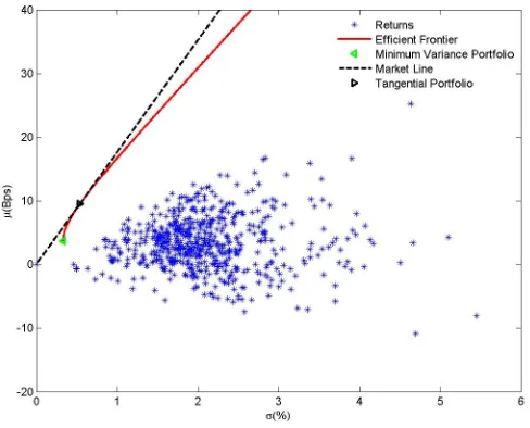
Figure (2.1) plots the efficient frontier for Eurostoxx constituent returns that have been computed from 2000 to 2010; the fully invested Maximum Sharpe
portfo-lio (or Tangential portfoportfo-lio); and the Minimum Variance portfoportfo-lio. Individually speaking, it can be seen that the assets are all sub-efficient (they all lie below
the efficient frontier); however, this is an illustration of the diversification benefit:
indeed, an efficient portfolio can be constituted of non-efficient assets.
Depend-ing on either their expected return or risk aversion, the investor can choose any
portfolio on the red curve.
2.2.3
Introduction of a risk-free asset
Assuming that the investor can freely borrow or lend money at a risk-free rate, denoted byrf: a proportion of the investor initial wealth can be borrowed or lent
at the risk-free rate. Thus, the portfolio optimisation problem for the investor
becomes:
minφ12φ0Σφ
2.2 The Efficient Frontier, Markowitz (1952)
Figure 2.1: Efficient Frontier
Proposition 2.5 (Efficient Frontier Equation with a risk-free asset). It is found that in the case where a risk-free asset exists, the Markowitz efficient frontier is a straight line with equation:
µP =√eσP +rf (2.4)
with e ≡(µ−rf1)0Σ−1(µ−rf1).
Proof. See Appendix.
2.2.3.1 Tangential portfolio
The Efficient Frontier line joins the risk-free rate with the Tangential
portfo-lio. The Tangential portfolio, denoted by φT, has coordinates that comply with
Equations (2.3) and (2.4).
Proposition 2.6 (Tangential Portfolio).
IfφT denotes the Tangential portfolio allocation; the mean and standard deviation of this portfolio are given by:
E(rφ T
) = √ e
ae−d+rf and V(r
φT
2.2 The Efficient Frontier, Markowitz (1952)
-where:
a=10Σ−11
b=10Σ−1µ=µ0Σ−11
c=µ0Σ−1µ d=ac−b2
e= (µ−rf1)0Σ−1(µ−rf1)
Proof. See Appendix.
2.2.3.2 The One Fund Theorem.
As any efficient portfolio lies on the efficient frontier line, it can be expressed in
terms of mean and variance as a linear combination of the Tangential portfolio
and the risk-free asset. This property is called the One Fund Theorem.
Theorem 2.2 (One Fund Theorem).
When a risk-free asset exists, the mean and variance of any efficient portfolio can be defined as a linear combination of any efficient portfolio (in particular the Tangential portfolio) and the risk-free asset.
Thus, the Markowitz frontier Equation becomes:
E(rφ P
) =rf +
(E(rφT)−r
f)
q
V(rφT)
q
V(rφP) (2.5)
Proof. Apply Equation (2.4) to the Tangential portfolio mean and variance.
This is illustrated in Figure (2.2), which sets rf = 1.5 basis points.
Extending from the Markowitz Efficient Frontier, Sharpe deduces an equilibrium
model that can be used to provide the correct price of a risky asset within the
framework of the mean-variance setting. The model is described in the following
2.3 The Capital Asset Pricing Model (CAPM), Sharpe (1964)
Figure 2.2: Efficient Frontier with a risk-free asset
2.3
The Capital Asset Pricing Model (CAPM),
Sharpe
(
1964
)
In what is considered to be a landmark paper, Sharpe (1964) extends the
Markowitz model to a multi-agent setting. Proposing a global equilibrium model,
known as the Capital Asset Pricing Model (CAPM), a mapping between risk, re-turn and asset prices is enabled. It is shown, that if all investors anticipate similar
expected returns and standard deviation of asset prices (and if the assumption
of the Markowitz model is satisfied), then all asset returns must lie on the
Secu-rity Market Line, which links expected return to risk. Thus, the CAPM gives a
standard of comparison under the strong consensus assumption that all investors
share the same view upon the distribution of asset returns.
The first sub-section will describe the Market portfolio and the Capital
Mar-ket Line, which effectively corresponds to the the Tangential portfolio and the
Markowitz Efficient Frontier described in Section 2.2.3. The equation of the equilibrium value for any risky asset in the context of the CAPM is then given.
2.3 The Capital Asset Pricing Model (CAPM), Sharpe (1964)
measure developed byJensen (1969). This allows the CAPM portfolio tested in
the following chapter to be constructed along with the Minimum Variance and
Maximum Sharpe portfolios described in the previous section.
2.3.1
The Capital Market Line (CML)
Assuming that investors rely on the mean-variance paradigm, and there is
com-plete agreement on the return distribution for the risky assets, it becomes possible
to compute a unique equilibrium price for any efficient portfolio. The Markowitz
frontier when computed for a representative agent, is from this point on referred
to as the Capital Market Line, and is considered to apply to all investors in the financial market. In addition, the Tangential portfolio has been renamed the
Market portfolio. Below, this portfolio will be described, after which the formal
equation of the Capital Market Line will be outlined.
2.3.1.1 The Market Portfolio
By reference to the One Fund Theorem (if a risk-free asset exists), it is known
that any investor can purchase a single portfolio, which is typically the Tangential
portfolio. In addition, the investor can freely borrow or lend money at a
risk-free rate to replicate any efficient portfolio. Furthermore, since in the CAPM
assumptions all investors use the same probability measure P to represent the risky assets distribution: the same representative portfolio will be considered.
This common ”One Fund” or representative portfolio is referred to as the Market
Portfolio. In actual fact, it represents a weighted average of all the risky assets
weighted by their proportional market capitalisation. This result is based on an equilibrium argument: if the representative portfolio were not identical for
investors sharing the same view on asset returns distribution, the price of assets
in higher demand would rise and the price of assets in lower demand would fall.
Ultimately, this will lead to a re-computation of the investors’ representative
portfolio converging towards the Market Portfolio. More formally, we have:
2.3 The Capital Asset Pricing Model (CAPM), Sharpe (1964)
Proof. The uniqueness of One Fund stems from the fact that all investors have identical anticipations about the distribution P; and therefore, solve the same optimisation problem as specified in section 2.2.3. The market capitalisation will be denoted by qi of the risky asset i, where i ∈[1, N] (i.e. the number of shares trading for the asset i multiplied by the price of the asset i). The Tangential portfolio allocation will be denoted byφT and the Market portfolio allocation by φM. According to the definition of the Market portfolio the following is given:
∀i∈[1, N], φM,i≡ q i
PN
i=1qi
Furthermore, it will be assumed that there areJ investors in the financial market. The amount detained by the investorj ∈[1, J], of any asseti∈[1, N], is denoted as θi,j. Therefore:
J
X
j=1
θi,j =qi
The total market capitalisation of the assetiis equal to the sum of the individual investments made by investors in the risky asset i. If the initial wealth of the investor j invested in the Tangential portfolioφT is denoted by xj0, the following is given:
J
X
j=1
xj0 =
N
X
i=1
qi
In fact, the sum of wealth invested in the risky assets must be equal to the total market capitalisation.
According to the One Fund Theorem the following is given:
∀i∈[1, N], θi,j =φT ,ixj0
Therefore, by summing over all the investors, the following is obtained:
∀i∈[1, N],
J
X
j=1
θi,j =φT ,i
J
X
j=1
xj0 ⇒φT ,i = q
i
PJ
j=1x
j
0
= q
i
PN
i=1qi
-which is precisely the allocation of the Market portfolio for the asset i.
The Market Portfolio is effectively the Market Index. Note: all tests carried out
in this research are run on European data, and the Market Index is taken to be
2.3 The Capital Asset Pricing Model (CAPM), Sharpe (1964)
2.3.1.2 The CML Equation
In the CAPM framework, the Efficient Frontier in the (σ−µ) map is a straight line,
emanating through the risk-free asset and passing through the Market portfolio.
The Efficient Frontier is then termed the Capital Market Line; the equation of
which is given by the following formula:
Proposition 2.8. The CML Equation shows the relation between the expected return and the risk of return for any efficient portfolio of assetsP. More formally, this is given as:
E(rφ P
) = rf +
(E(rφM)−r
f)
q
V(rφM)
q
V(rφP) (2.6)
Proof. This is a direct consequence of the One Fund Theorem as applied to the Market Portfolio.
The expected return of any efficient portfolio belonging to the CML is a linear
function of its standard deviation. The slope factor: E(rφ
M
)−rf √
V(rφM
) is called the market
price of risk. To simplify notations in the following, instead of rφM, the Market
portfolio returns are denoted by rM .
2.3.2
The Security Market Line (SML)
The CAPM goes further, and signifies how the expected return of a single asset
should relate to its individual risk. This gives a precise pricing formula for any
risky asset in the CAPM framework. The price of risk is commonly referred to
as Beta, as shown in a first sub-section. The Security Market Line Equation and
pricing formula for any risky asset are given in a subsequent section.
2.3.2.1 The CAPM Betas
2.3 The Capital Asset Pricing Model (CAPM), Sharpe (1964)
βi,M = COV(r
i,rM)
V(rM)
The Beta of an asset i represents the relative contribution of the asset return i
to the variance of the market return rM.
2.3.2.2 The SML Equation
The main result of the CAPM is that Sharpe extends the CML to a general
relationship between any single risky asset expected return (that is not necessarily
efficient and therefore does not lay automatically on the CML) and the Market
portfolio return:
Proposition 2.9 (Security Market Line Equation). The expected return of any asset i is given by:
E(ri) =rf +βi,M[E(ri)−rf]
Proof.
The portfolio a constituted by the risky asset i in proportion a, and the market portfolio in proportion (1-a) will be considered. The first two moments of this portfolio are expressed as:
E(ra) =aE(ri) + (1−a)E(rM)
V(ra) =a2V(ri) + (1−a)2V(rM) + 2a(1−a)COV(ri, rM)
Thus, it is found that:
(
dE(ra)
da =E(r i)−
E(rM) dV(ra)
da = 2[aV(r
i) + (a−1)
V(rM) + (1−2a)COV(ri, rM)]
When a= 0 is taken:
dpV(ra)
da
a=0 =
1
2pV(ra)
dV(ra)
da
COV(ri, rM)−V(rM)
p
2.3 The Capital Asset Pricing Model (CAPM), Sharpe (1964)
And then:
dE(ra) dpV(ra)
a=0 =
(E(ri)−
E(rM))pV(rM) COV(ri, rM)−V(rM)
Using equality with the CML slope in a= 0, the result is finally:
(E(ri)−E(rM))
√
V(rM) COV(ri,rM)−
V(rM) =
E(ri)−rf
√
V(rM)
Under the equilibrium conditions assumed by the CAPM, any asset (including
efficient assets) should fall on the Security Market Line. Therefore, under the
CAPM assumptions, the Security Market Line is a universal pricing line.
2.3.3
The CAPM
The CAPM proposes a model for asset price returns that complies with the SML. In a first sub-section, the CAPM will be formally described, and then the method
of building the CAPM portfolio based on the Jensen measure will be presented.
The CAPM portfolio will be empirically tested in Chapter3, among other classical portfolios.
2.3.3.1 The CAPM Equation
The CAPM states that any random asset return ri can be separated into a
sys-tematic component and a residual component:
ri =rf +βi(rM −rf) +i
If no assumption is made on the distribution of i, this equation is arbitrary.
To be coherent with the SML (taking the expected value on both sides of the equation), the CAPM assumes that the idiosyncratic risk is uncorrelated with
the market risk, and its expected value is zero. The CAPM theorem can now be
2.3 The Capital Asset Pricing Model (CAPM), Sharpe (1964)
Theorem 2.3 (CAPM). Any risky asset return can be expressed with respect to its price for risk:
ri =rf +βi(rM −rf) +i
-where i is such that:
∀i, E(i) = 0 and ∀i,
COV(i, rM) = 0
This leads to the following:
∀i, E(ri) = βiE(rM) and ∀i, V(ri) = (βi)2V(rM) +V(i)
To summarise the workings undertaken in the chapter so far, the CAPM de-composes any risky asset excess return in a systematic component, defined as
βi(rM −r
f), and an idiosyncratic component, which is defined as i. The first
equation states that the expected return of a risky asset is the product of the
risky asset Beta and the expected return of the market. This relation defines
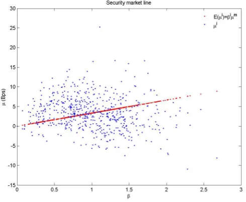
the ”Security Market Line”. Figure (2.3) plots the Security Market Line for the Eurostoxx 600 constituents (the Betas are estimated over the whole period
Jan-uary 2000 to April 2010). It can be observed that the CAPM relationship is not
well respected empirically (the empirical observations presented are well dispersed
around the theoretical SML...). The second equation states that any asset risk
can be decomposed into a systematic risk (the market risk adjusted by the asset Beta) and a specific risk. Under the CAPM assu