SRC Technical Note
1998 - 001
February 8, 1998
On the Analysis of Randomized Load Balancing Schemes
Michael Mitzenmacher
d i g i t a l
Systems Research Center130 Lytton Avenue Palo Alto, California 94301
http://www.research.digital.com/SRC/
On the Analysis of Randomized Load Balancing Schemes
Michael Mitzenmacher
∗Abstract
It is well known that simple randomized load balancing schemes can balance load effectively while incurring only a small overhead, making such schemes appealing for practical systems. In this paper, we provide new analyses for several such dynamic randomized load balancing schemes.
Our work extends a previous analysis of the supermarket model, a model that abstracts a simple, efficient load balancing scheme in the setting where jobs arrive at a large system of parallel processors. In this model, customers arrive at a system of n servers as a Poisson stream of rateλn,λ <1, with service requirements exponentially distributed with mean 1. Each customer chooses d servers independently and uniformly at random from the n servers, and is served according to the First In First Out (FIFO) protocol at the choice with the fewest customers. For the supermarket model, it has been shown that using d=2 choices yields an exponential improvement in the expected time a customer spends in the system over d =1 choice (simple random selection) in equilibrium. Here we examine several variations, including constant service times and threshold models, where a customer makes up to d successive choices until finding one below a set threshold.
Our approach involves studying limiting, deterministic models representing the behavior of these systems as the number of servers n goes to infinity. Results of our work include useful general theorems for showing that these deterministic systems are stable or converge exponentially to fixed points. We also demonstrate that allowing customers two choices instead of just one leads to exponential improve-ments in the expected time a customer spends in the system in several of the related models we study, reinforcing the concept that just two choices yields significant power in load balancing.
1
Introduction
Distributed computing systems continue to rise in prevalence; networks of workstations and clusters of personal computers hold the promise of increased power and price/performance ratios. It has long been known that in distributed systems, redistributing the workload through load balancing can lead to significant performance improvements, in terms of both the mean and standard deviation of the time jobs spend in the system (for example, see [7, 35]). Moreover, simple randomized schemes with low overhead have proven effective in simulations; however, analyzing such schemes is often difficult. In this paper, we provide new analyses for several dynamic randomized load balancing models. Unlike previous similar analyses, we do not assume that in equilibrium each server is stochastically independent from other servers.
One example of the type of problem we consider, previously studied in [27], is the following natural dy-namic model: customers arrive as a Poisson stream of rateλn, whereλ <1, at a collection of n servers. The service times for the customers are independent and exponentially distributed with mean 1. Each customer chooses some constant number d of servers independently and uniformly at random from the n servers, and waits for service at the one currently containing the fewest customers (ties being broken arbitrarily), accord-ing to the First In First Out (FIFO) protocol. We call this model the supermarket model, or the supermarket
∗This work was supported in part by the ONR and in part by NSF Grant CCR-9505448. Much of this work was done while the
author was a student at U.C. Berkeley. A previous version of this work appeared in the 9th ACM Symposium on Parallel Algorithms
B A
Figure 1: The supermarket model. Incoming customer A chooses two random servers, and queues at the shorter one. Customer B has recently been served and leaves the system.
system (see Figure 1). We are interested in the behavior of this system in equilibrium. Note that the average
arrival rate per queue is less than service rate (λ <1), we expect the system to be stable, in the sense that the expected number of customers per queue remains finite in equilibrium.
Standard queueing theory does not directly apply to the supermarket model, because the server loads are dependent: the arrival rate at any server depends on the loads at the other servers. This dependency complicates the analysis dramatically.
Many variations on the supermarket model exist. For example, in a threshold system, an incoming cus-tomer successively chooses queues at random until either finding one with a load below a fixed threshold or using d choices. A threshold scheme may be more efficient than giving each customer d choices in practice, since each choice will generally require some communication, and threshold schemes reduce the amount of necessary communication. As another example, service times might not be eponentially distributed, but constant, or given by another distribution. In this paper, we introduce new analyses for these and other variations. Our approach, following that of [27], has two main components:
• We define an idealized process, corresponding to a system with an infinite number of servers. We then
analyze this process, which is cleaner and easier because its behavior is completely deterministic.
• We relate the idealized system to the finite system, bounding the error between them.
Our analysis of the limiting system (as the number of servers grows to infinity) focuses on finding the
fixed point (or equilibrium point) to which the system tends. If the system converges to its fixed point, then
we can use it to determine such quantities as the expected time a customer spends in the system. For most of the idealized systems we consider, we show exponential convergence to the fixed point, which demonstrates that the system approaches the fixed point very quickly. Indeed, besides determining the behavior of several interesting systems, a major contribution of this work is a simple, general theorem that gives appropriate conditions for convergence; we expect this theorem will prove useful in other settings as well. We also demonstrate through simulations that the method provides accurate numerical estimates of performance, even when the actual number of servers is relatively small.
even the simple systems we study demonstrate remarkably interesting behavior. In particular, we emphasize throughout that there is often a qualitative difference between systems where customers choose a single des-tination randomly and systems where customers have two or more choices available, leading to exponential improvement in measures such as the expected time in the system. Hence our work extends a great deal of previous work demonstrating the power of two choices in load balancing to several new settings, providing further evidence of the significance of this idea in the design of distributed systems.
1.1
Previous work
Distributed load balancing strategies where individual customer decisions are based on information about a limited number of other processors have been studied analytically by Eager et al. [7, 8, 9] and through trace-driven simulations by Zhou [35]. In fact, Eager et al. also use Markovian models for their analysis [7, 8, 9]; however, the authors derive their results assuming that the state of each queue is stochastically independent of the state of any other queue. This approach is exact in the asymptotic limit as the number of queues grows to infinity. Our work avoids these assumptions and introduces several new directions in the analysis of these systems. Zhou’s work examines the effectiveness of the load balancing strategies proposed by Eager
et al. as well as others in practice using a trace-driven simulation. Both Eager et al. and Zhou suggest that
simple randomized load balancing schemes, based on choosing from a small subset of processors, perform extremely well.
In another well-studied model, incoming customers join the shortest queue; see, for example, the work by Adan, van Houtum, and van der Wal [1] and by Adan, Wessels, and Zijm [2, 3] for results and further references. The shortest queue model appears more applicable to centralized systems, whereas the limited coordination enforced by our model corresponds nicely to models of distributed systems.
Randomized load balancing schemes have also been analyzed in the static case, where there are a fixed number of customers to be permanently distributed, as in a static hash table. For example, Karp, Luby, and Meyer auf der Heide showed that using two hash functions instead of one could provide an exponential improvement in the maximum load of a hash bucket [13]; this idea was further developed and aanalyzed by Azar, Broder, Karlin, and Upfal [5]. Our work demonstrates that making two choices leads to a similar exponential improvement in the dynamic setting as well.
The justification of the relationship between the finite and limiting systems relies on Kurtz’s work on
density dependent jump Markov processes [10, 19, 20, 21, 22]. Because Kurtz’s work is rather technical,
we only briefly describe it here, focusing instead on examining a variety of models and attempting to gain insight into the load balancing problem. More details regarding the application of Kurtz’s work these models can be found in [28]. This approach has been used similarly in several other works (for example, see [4, 11, 14, 15, 27, 31, 33, 34]).
2
The supermarket model
In this section, we review results for the supermarket model from [27]. This review allows us to introduce the necessary terminology and methodology that we will use to study other systems.
2.1
The limiting system
Recall the definition of the supermarket model: customers arrive as a Poisson stream of rateλn, whereλ <1,
at a collection of n FIFO servers. Each customer chooses some constant d ≥ 2 servers independently and
uniformly at random with replacement1 and queues at the server currently containing the fewest customers.
The service time for a customer is exponentially distributed with mean 1.
We define mi(t)to be the number of queues with at least i customers at time t, and si(t)=mi(t)/n to be fraction of queues with at least i customers. We drop the reference to t in the notation where the meaning
is clear. In an empty system, which corresponds to one with no customers, s0=1 and si =0 for i ≥1. We
can represent the state of the system at any given time by an infinite dimensional vectorEs =(s0,s1,s2, . . .).
It is clear that for each value of n, the supermarket model can be considered as a Markov chain on the above state space.
We now introduce a deterministic limiting system related to the finite supermarket system, given by the following set of differential equations:
dsi
dt = λ(s
d
i−1−sid)−(si −si+1) for i ≥1;
s0 = 1.
(1)
To explain the reasoning behind the system (1), we determine the expected change in the number of servers with at least i customers over a small period of time of length dt. The probability a customer arrives during this period isλn dt, and the probability an arriving customer joins a queue of size i−1 is sid−1−sid. (This is the probability that all d servers chosen by the new customer are of size at least i−1, but not all are of size at least i .) Thus the expected change in mi due to arrivals is exactlyλn(sid−1−sid)dt. Similarly, the probability a customer leaves a server of size i in this period is nidt =n(si −si+1)dt. Hence, if the system
behaved according to these expectations, we would have
dsi
dt =
1
n · dmi
dt =λ(s
d i−1−s
d
i )−(si −si+1).
It should be intuitively clear that as n → ∞the behavior of the supermarket system approaches that of this
deterministic system; this is justified by Kurtz’s theorem, as explained in Appendix A. For now, we simply take this set of differential equations to be the appropriate limiting process.
2.2
The fixed point
Given a reasonable condition on the initial point Es(0), the infinite process described by the system (1)
converges to a fixed pointπE such that ifEs(t)= EπthensE(t0)= Eπfor all t0≥t. For the supermarket model a
necessary and sufficient condition forEs to be a fixed point is that for all i , dsi
dt|πE =0.
Lemma 1 [[27], Lemma 1.] The system (1) with d ≥2 has a unique fixed point withP∞i=1πi <∞given
byπi =λ
di−1
d−1.
Definition 2 A sequence(xi)∞i=0 is said to decrease doubly exponentially if and only if there exist positive constants N, α <1, β >1, andγ such that for i ≥ N , xi ≤γ αβ
i .
It is worth contrasting the result of Lemma 1 with the case where d = 1 (i.e., all servers are M/M/1
queues), for which the fixed point is given byπi =λi. For d = 2, the fixed point is given byπi =λ2
i−1
.
The key feature of the supermarket system is that for d ≥2 the tailsπi decrease doubly exponentially, while
for d =1 the tails decrease only geometrically (or singly exponentially).
2.3
Convergence to the fixed point
The deterministic differential equations (1), along with an initial point, define a trajectory of the system in the infinite dimensional space. In [27] it was shown that every trajectory of the limiting model of the
supermarket system converges to the fixed pointπE =(πi)of Lemma 1 in an appropriate metric. We review
the main points here. In what follows we assume that d ≥2 unless otherwise specified.
To show convergence, we find a suitable potential function (also called a Lyapunov function in the
dynamical systems literature) 8(t). The potential function must be related to the distance between the
current point on the trajectory and the fixed point; by showing the potential function decreases quickly over time, we may show the trajectory heads towards the fixed point. A natural potential function to consider is
D(t)=P∞i=1|si(t)−πi|, which measures the L1-distance (or Manhattan distance) between the two points.
The potential function used in [27] is actually a weighted variant of this, namely8(t)=P∞i=1wi|si(t)−πi| for suitably chosen weightswi.
The supermarket system not only converges to its fixed point, but that it does so exponentially.
Definition 3 The potential function 8is said to converge exponentially to 0, or simply to converge expo-nentially, if8(0) <∞and8(t)≤c0e−δt for some constantδ >0 and a constant c0which may depend on the state at t =0.
Exponential convergence implies not only that the limiting system approaches the fixed point, but that it does so rapidly, making it a suitable reference point for system performance in practice.
Theorem 4 [[27], Theorem 6] Let8(t)=P∞i=1wi|si(t)−πi|, where for i ≥1,wi ≥1 are appropriately
chosen constants. If8(0) <∞, then8converges exponentially to 0. In particular, if there exists a j such that sj(0)=0, then8converges exponentially to 0.
The condition of Theorem 4 that there exists a j such that sj(0)=0 is a natural one. It can be interpreted as saying initially there is an upper bound on the maximum queue size.
Corollary 5 [[27], Corollary 7] Under the conditions of Theorem 4, the L1-distance from the fixed point D(t)=P∞i=1|si(t)−πi|converges exponentially to 0.
Corollary 5 shows that the L1-distance to the fixed point converges exponentially quickly to 0. Given
this convergence, we may now ask what the expected time in the system looks like. It is interesting to
compare the case where d ≥2 to the case of d =1 (for which the expected time is well known).
Theorem 6 [[27], Theorem 8] The expected time a customer spends in the limiting model of an initially empty supermarket system for d ≥2 converges as t → ∞to Td(λ)≡
P∞
i=1λ di−d
d−1. If T1(λ)≡ 1
1−λ, then for
λ∈[0,1], Td(λ)≤cd(ln T1(λ))for some constant cd dependent only on d. Furthermore, limλ→1− ln TTd(λ)1(λ) =
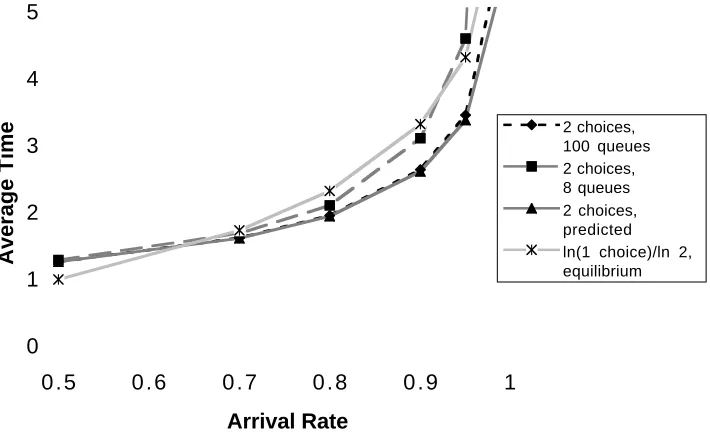
0 1 2 3 4 5
0 . 5 0 . 6 0 . 7 0 . 8 0 . 9 1
Arrival Rate
Average Time
2 choices, 100 queues 2 choices, 8 queues
[image:7.612.126.481.73.290.2]2 choices, predicted ln(1 choice)/ln 2, equilibrium
Figure 2: The graph compares the expected time in the system from simulations of 8 and 100 queues with the limiting system prediction when two choices are made and the logarithm of the expected time in equilibrium when one choice is made under various arrival rates (λ).
Choosing from d > 1 queues hence yields an exponential improvement in the expected time a customer
spends in the limiting system, and as λ → 1− the choice of d affects the time only by a small constant
factor (dependent on d). These results are remarkably similar to those for the static load balancing problem studied in [5].
Simulations verify that this behavior is apparent even in small systems; for example, see Figure 2. More details are given [27] or [28].
3
Constant service times
The assumptions underlying the supermarket model, namely that the arrival process is Poisson and that the service times are exponentially distributed, do not accurately describe many (and probably most) real systems, although they are useful because they lead to a simple Markovian system. In this section, we demonstrate how to modify our approach to handle more general service and arrival times. We focus on the example where the service time is a fixed constant. The approach we use is based on Erlang’s method
of stages, which we shall describe briefly here. For a more detailed explanation see [17, Sections 4.2 and
4.3]. We approximate the constant service time with a gamma distribution: a single service will consists
of r stages of service, where each stage is exponentially distributed with mean 1/r . As r becomes large,
the expected service time remains 1 while the variance falls like 1/r , so that the service time behaves like a
constant random variable in the limit as r → ∞.
The state of a queue will now be the total number of stages remaining that the queue has to
pro-cess, rather than the number of customers; that is, the state of a queue is [r(# of waiting customers)+
stages of the customer being served].Since r determines the size of the state space, numerical calculations
will be easier if we choose r to be a reasonably small finite number. Our simulations suggest that for r ≈20
There is some ambiguity in the meaning of a customer choosing the shortest queue. If the number of customers in two queues are the same, can an incoming customer distinguish which queue has fewer stages of service remaining? Let us first consider the case where we have aware incoming customers, who can tell
how many stages are left for each of their d choices and choose accordingly. Let sj be the fraction of queues
with at least j stages left to process (where we take sj =1 whenever j ≤0). Then sj increases whenever an
arrival comes to a queue with at least j−r and fewer than j stages left to complete. Similarly, sj decreases whenever a queue with j stages completes a stage, which happens at rate r . The corresponding system of differential equations is thus
dsj
dt =λ(s
d j−r−s
d
j)−r(sj −sj+1).
(When r =1, this corresponds exactly to the standard supermarket model.)
We can identify a unique fixed pointπE for this system (usingdsj
dt =0 at the fixed point). We must have
π1=λ(intuitively because the arrival rate and exit rate of customers must be equal), andπi =1 for i ≤0.
From these initial conditions one can find successive values ofπj from the recurrence
πj+1=πj− λ(πd
j−r−πjd)
r . (2)
Unfortunately, we have not found a convenient closed form forπj.
We say that the system has unaware customers if customers learn only the queue size of their choices, and not the number of stages. If more than one server chosen by an incoming customer has the shortest queue, then the customer chooses randomly from those servers. The differential equations are slightly more
complicated than in the aware case. Again, let sj be the fraction of queues with at least j stages left to
process. For notational convenience, let Si = s(i−1)r+1 be the fraction of queues with at least i customers
(where S0 = 1 always), and let φ(j) = drjebe the number of customers in a queue with j stages left to
process. The corresponding differential equations are:
dsj
dt = λ(S
d
φ(j)−1−S
d
φ(j))
sj−r−Sφ(j)
Sφ(j)−1−Sφ(j) + λ(Sdφ(j)−Sφ(d j)+1) Sφ(j)−sj
Sφ(j)−Sφ(j)+1 −
r(sj −sj+1).
Note that the fixed point cannot be determined by a simple recurrence, as the derivative of sj depends
on Sφ(j),Sφ(j)−1, and Sφ(j)+1. One can find the fixed point to a suitable degree of accuracy by standard
numerical methods, however.
3.1
Constant versus exponential service times
The question of whether constant service times reduce the expected delay in comparison to exponential service times often arises when one tries to use standard queueing theory results to find performance bounds on networks. (See, for example, [12, 25, 26, 29, 32].) Generally, results comparing various service times are achieved using stochastic comparison techniques. Here, we instead compare the fixed points of the corresponding limiting systems.
We show that at the fixed points, the fraction of servers with at least k customers is greater when service
times are exponential than when service times have a gamma distribution (with r ≥ 2) with the same
times with exponential service times with this approach requires technical arguments regarding changing
the order in which the limits as n→ ∞and r → ∞are taken; for example, see [31, Chapter 14]. We have
not completed such a formal justification. However, the theorem below is the key step in the argument, and moreover it is interesting in its own right.)
We consider the case of aware customers where service times have a gamma distribution corresponding to r stages. Recall that the fixed point was given by the recurrence (2) asπj+1=πj−λ(πjd−r−πjd)/r , with
π1 = λand πi = 1 for i ≤ 0. The fixed point for the standard supermarket model, as found in Lemma 1,
satisfies πi+1 = λπid. Sinceπ1 isλin both the standard supermarket model and the model with gamma
distributed service times, to show that the tails are larger in the standard supermarket model, it suffices to
show that πφ(j)+1 ≤ λπφ(d j) in the aware customer model. Inductively it is easy to show the following
stronger fact:
Theorem 7 In the system with aware customers, for j ≥1,
πj = λ
r
j−1
X
i=j−r πd
i .
Proof: The equality can easily be verified for 1 ≤ j ≤ r . For j > r , the following induction yields the
theorem:
πj = πj−1−λ r(π
d
j−r−1−πjd−1)
= πj−2−λ r(π
d
j−r−1+πjd−r−2−πjd−1−πjd−2)
...
= πj−r−λ
r
j−Xr−1
i=j−2r
πd i −
j−1
X
k=j−r πd
k !
= λ
r
j−1
X
k=j−r πd
k.
Here the last step follows from the inductive hypothesis, and all other steps follow from the recurrence equation (2) for the fixed point.
An entirely similar proof holds even in the case of unaware customers [28, Theorem 4.7].
3.2
Simulations and other service times
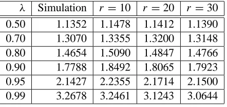
We show with simulations that small values for the number of stages r yield good approximations for constant service times. Table 1 compares the value of the expected time a customer spends in a limiting
system with unaware customers and d =2 choices per customer obtained using various values of r against
the results from simulations with constant service times for 100 queues. The simulation results are the average of ten runs, each for 100,000 time units, with the first 10,000 time units excluded to account for the fact that the system begins empty. In all cases exceptλ=0.99 increasing r yields a better match between the
simulation and the prediction from the fixed point; this discrepancy is because the predictions forλ=0.99
are not sufficiently accurate for systems of only one hundred queues.
λ Simulation r =10 r =20 r =30
0.50 1.1352 1.1478 1.1412 1.1390
0.70 1.3070 1.3355 1.3200 1.3148
0.80 1.4654 1.5090 1.4847 1.4766
0.90 1.7788 1.8492 1.8065 1.7923
0.95 2.1427 2.2355 2.1714 2.1500
[image:10.612.197.418.71.175.2]0.99 3.2678 3.2461 3.1243 3.0644
Table 1: Simulations versus estimates for constant service times: 100 queues.
positive random variable can be approximated arbitrarily closely by a mixture of countably many gamma distributions [16, Lemma 3.9]. In practice, for the solution of this problem to be computable in a reasonable amount of time, both the number of distributions in the mixture and the number of stages for each distribution must be small in order to keep the total number of states reasonably small. Although these limitations appear severe, many service distributions can still be handled easily. For example, as we have seen, in the case of constant service times one only needs to use a single gamma distribution with a reasonable number of stages r to get a very good approximation. This increases the state space, and hence approximately the time to determine the behavior of the linear equations, by a factor of r over the case where service times are exponential. Distributions where the service time takes on one of a small finite number of values can be handled similarly.
4
Other dynamic models
In this section, we shall develop limiting systems for some variations on the supermarket model and show that many of these systems also converge exponentially to their fixed points. (As all of the systems we examine have a unique fixed point where the average number of customers per queue is finite, we shall simply refer to the fixed point for these systems.)
4.1
Customer types and errors
One way to extend the supermarket model is to consider what happens when different customers can have different numbers of choices. We will observe that giving even a small fraction of customers an extra choice can have a dramatic effect on load distribution, especially in a heavily loaded system. This fact has important practical ramifications; for example, since obtaining load information typically requires sending messages through the system, one may wish to reduce the average number of messages per customer by only giving a fraction of the customers additional choices.
We examine the specific case where there are two types of customers. One type chooses only one queue;
each customer is of this type with probability 1−p. The more privileged customer chooses two queues;
each customer is of this type with probability p. The corresponding limiting system is governed by the following set of differential equations:
dsi
dt = λp(s 2
i−1−si2)+λ(1−p)(si−1−si)−(si −si+1). (3)
The fixed point is given byπ0 =λ,πi =λπi−1(1− p+ pπi−1). Note that this matches the supermarket
model for d =1 and d =2 in the cases where p=0 and p =1, respectively. There does not appear to be
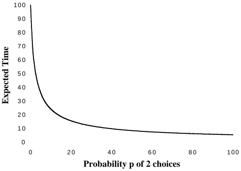
0 1 0 2 0 3 0 4 0 5 0 6 0 7 0 8 0 9 0 1 0 0
0 2 0 4 0 6 0 8 0 1 0 0
Probability p of 2 choices
[image:11.612.181.430.71.248.2]Expected Time
Figure 3: Expected time in the system versus probability (p) of that a customer chooses two locations
(λ=0.99).
As shown in Figure 3, which demonstrates the results for the limiting system, the effect of increasing the fraction of customers with two choices has a non-linear effect on the expected time that is dramatic at
high loads; atλ = 0.99, most of the gain occurs when only 20% of the customers have two choices. Our
simulation results verify that the behavior of finite systems accurately matches the behavior predicted by our limiting model.
This model has an interesting alternative interpretation. A customer who only has one choice is equiva-lent to a customer who has two choices, but erroneously goes to the wrong queue half of the time. Hence, the above system is equivalent to a two-choice system where customers make errors and go to the wrong queue
with probability 1−2p. A model of this sort may therefore also be useful in the case where the information
available to the customers from the chosen servers is unreliable or approximate. This analysis suggests that as long as this approximate load information reflects server loads with some reasonable accuracy between updates, choosing from two servers should still perform quite well. (See also [24] for similar ideas in other scenarios.)
4.2
Closed models
In the closed supermarket model, at each time step exactly one non-empty queue, chosen uniformly at ran-dom, completes service, and the customer is immediately recycled back into the system by again choosing
the shortest of d random queues. Let the number of customers that cycle through the system beαn. Note
that the average number of customers per queue isα; this corresponds to the invariantP∞i=1si =α. The limiting system is again very similar to that of the original supermarket model. An important difference is that at each step, the probability that a customer leaves a server with i customers is si−si+1
s1 ,
since a random queue with at least one customer loses a customer. The corresponding differential equations are thus
dsi
dt =s
d
i−1−sid−
si −si+1 s1
. (4)
To find the fixed point, assumeπ1 =β. Then inductively, we can solve to findπi = β
di−1
d−1; the correct
value ofβcan be found by using the constraintP∞i=1πi =
P∞
i=1β di−1
4.3
Bounded buffers
In practice, we may have a system where the queue size has a maximum limit, say b. For example, if customers are processes with associated data, then the queue size may be limited by the amount of memory in a server’s buffer. In this case, we assume that arriving customers that find queues filled are turned away. That is, for the supermarket model, if an arriving customer chooses d queues that all have b customers already waiting, the customer leaves the system unserved immediately.
The state can be represented by a finite dimensional vector(s0,s1, . . . ,sb). The long-term probability
that a customer is turned away can be determined by finding from the point, and isπbd. The limiting system
is given by the following equations:
dsi
dt = λ(s
d
i−1−sid)−(si −si+1) , i<b; dsb
dt = λ(s
d
b−1−sdb)−sb.
Note that at the fixed point for this problem,π16=λ. The total arrival rate of customers into the queues
at the fixed point isλ(1−πbd), as some customers do not enter the system. Since at the fixed point the total
rate at which customers arrive must equal the rate at which they leave, we have π1 = λ(1−πbd). Using
the differential equations, we can develop a recurrence for the values of the fixed pointπi. This recurrence
yields a polynomial equation forπb, which can be shown to have a unique root between 0 and 1. Solving
forπbthen allows us to compute the fixed point numerically.
4.4
Convergence and stability of limiting systems
In this section, we provide a general theorem (similar to Theorem 4) that can be used to show that several systems we have considered converge exponentially to their fixed point. In some cases, however, proving convergence is difficult. Instead of proving convergence, it is often easier to prove the weaker property of
stability of the fixed point. We will say that a fixed point is stable if the L1-distance to the fixed point is non-increasing along every trajectory (this is actually stronger than the standard definition). We also give a general theorems with conditions for stability. We believe these results are interesting in their own right and will be useful in the future for studying other systems. (For another approach to proving convergence for these problems, see [33].)
We consider general systems governed by the equationsdsi
dt = fi(Es)for i ≥1, with fixed pointπE =(πi). Leti(t)=si(t)−πi, with the understanding that for i <1 or i larger than the dimension of the state space
we fixi =0. We shall drop the explicit dependence on t when the meaning is clear. For convenience, we
shall consider only systems where si(t) ∈ [0,1] for all t, and hencei(t) ∈ [−πi,1−πi] for all t. This restriction simplifies the statements of our theorems and can easily be removed; however, all the systems described in this section meet this condition.
We examine the L1-distance D(t)=
P
i≥1|i(t)|. In the case where our state space is countably infinite dimensional, the upper limit of the summation is infinity, and otherwise it is the dimension of the state space. For technical reasons, we letd Ddt denote the right-hand derivative (this will be explained in the last paragraph of the proof). We shall prove that d Ddt ≤ 0 everywhere; this implies that D(t)is non-increasing over time, and hence the fixed point is stable.
For many of the systems we have examined, the functions fihave a convenient form: they can be written
as sums of polynomial functions of the individual sj, with no product terms sjsk for j 6=k. This allows us
to group together terms in d D/dt containing only i, and consider them separately. By telescoping the
Theorem 8 Suppose we are given a system di/dt = P
j gi,j(j), where the functions gi,j satisfy the
following conditions:
1. gi,i(x)= − P
j6=igj,i(x)for x ∈[−πi,1−πi];
2. for all i 6= j , sgn(gj,i(x))=sgn(x)for x ∈[−πi,1−πi].
Then for D(t)=P∞i=1|i(t)|we have d D/dt ≤0, and hence the fixed point is stable.
Proof:
For each i , we group the terms in i of d D/dt, and show that the sum of all terms involving i is at
most 0. Note that, technically, d D/dt is not well-defined when somei =0; we shall clarify this problem
subsequently and temporarily we assume that alli are non-zero.
The terms containingi in d D/dt sum to h(i)=gi,i(i)sgn(i)+ P
j6=igj,i(i)sgn(j). By condition
2 of the statement of the theorem, h(i) is maximized when sgn(j) = sgn(i) for all j 6= i . Hence
h(i) ≤ sgn(i) P
j gj,i(i) = 0, where the last equaity follows from condition 1 of the theorem. Hence
d D/dt ≤0, and this suffices to show that the fixed point is stable.
We now consider the technical problem of defining d D/dt wheni(t) = 0 for some i . Since we are
interested in the forward progress of the system, it is sufficient to consider the upper right-hand derivatives ofi. (See, for instance, [23, p. 16].) That is, we may define
d|i|
dt
t=t0
≡ lim t→t0+
|i(t)|
t−t0,
and similarly for d D/dt. Note that this choice has the following property: ifi(t) =0, then ddt|i| t=t0
≥ 0,
as it intuitively should be. The above proof applies unchanged with this definition of d D/dt, with the
understanding that with regard to the sgn function the case i > 0 includes the case where i = 0 and
di/dt≥0, and similarly the casei <0 includes the case wherei =0 and di/dt <0.
It is simple to check that the conditions of Theorem 8 hold for several of the systems we have studied. Hence we immediately have the following corollary:
Corollary 9 The limiting systems for the following systems have stable fixed points: gamma distributed service times with aware customers (Section 3), customer types (Section 4.1), and bounded buffers (Sec-tion 4.3).
Proof: We consider only the system with customer types described in Section 4.1 and whose behavior is
given by equation (3), as the argument is entirely similar for the other models stated. With the substitutioni =si−πi, equation (3) becomes
di
dt = −2λpπii−λp 2
i −λ(1− p)i−i +2λπi−1i−1+λi2−1+λ(1−p)i+1+i+1. (5)
(Note that all terms without somej factor sum to 0 by definition of the fixed point.)
Condition 1 of Theorem 8 clearly holds from equation (5). Condition 2 is also easily checked– note that sgn(i−1=sgn(λi2−1+2λπi−1i−1)over the appropriate interval. Hence the conditions of Theorem 8 hold,
proving the corollary.
Theorem 10 Suppose we are given a system di/dt = P
gi,j(j), and suppose also that there exists an
increasing sequence of real numberswi (withw0 =0) and a positive constantδ such that thewi and the
functions gi,j satisfy the following conditions:
1. sgn(x)Pjwjgj,i(x)≤ −δwi|x|for x∈[−πi,1−πi];
2. for all i 6= j , sgn(gj,i(x))=sgn(x)for x ∈[−πi,1−πi].
Then for8(t) = P∞i=1wi|i(t)|, we have that d8/dt ≤ −δ8, and hence from any initial point where P
iwi|i|<∞the process converges exponentially to the fixed point in L1-distance.
Proof: We group the terms ini from d8/dt as in Theorem 8. By the assumptions of the theorem, the sum of all the terms involvingi is at most−δwi|i|. We may conclude that d8/dt ≤ −δ8(t)and hence8(t)
converges exponentially to 0. Also, note that we may assume without loss of generality thatw1 =1, since
we may scale thewi. Hence we may take8(t)to be larger than the L1-distance to the fixed point D(t), and
thus the process converges exponentially to the fixed point in L1-distance.
Proving convergence thus reduces to showing that a suitable sequence of weightswi satisfying Condition
1 of Theorem 10 exist, which is quite often straightforward. In fact, Theorem 10 applies directly to several of the models we have mentioned. For these models we will assume, as in Theorem 4, that in our intial state there exists an upper bound on the initial queue size, to guarantee that the system begins in a well-defined state.
Corollary 11 The limiting systems for the following systems converge exponentially to their fixed points: gamma distributed service times with aware customers (Section 3), customer types (Section 4.1), and bounded buffers (Section 4.3).
Proof: Again we consider only the system with customer types given by equation (3), as the argument for
other models is similar. That Condition 2 of Theorem 10 holds was shown in Corollary 9. Hence we need
only show that a δ and a sequencewi that satisfies Condtion 1 of Theorem 10 exist. We setw0 = 0 and
w1=1 and show how to define the otherwi and theδaccordingly.
Using equation (5), Condition 1 of Theorem 10 becomes the following:
sgn(i)
wi+1(2λpπii +λpi2)−wi(2λπii +λi2+λ(1−p)i +i)+wi−1(λ(1−p)i +i)
≤ −δwi|i|
As|i| =sgn(i)i, and the condition trivially holds ifi =0, we may divide through by|i|to restate the condition as
(wi−wi−1)(1+λ(1−p))+(2λpπi +λpi)(wi −wi+1)≥δwi;
or, using the fact that|i| ≤1,
wi+1≤wi +wi(
1+λ(1−p)−δ)−wi−1(1+λ(1−p))
λp(2πi+1)
.
It is simple to check inductively that one can choose an increasing sequence ofwi (starting withw0 =
0, w1 =1) and aδsuch that thewi satisfy the above restriction. For example, we break the terms up into
two subsequences. The first subsequence consists of allwi such thatπi satisfiesλp(2πi +1) ≥ 1+2λ. For these i we can choosewi+1 =wi +wi(1−δ)3−wi−1. Because this subsequence has only finitely many terms,
we can choose a suitably smallδso that this sequence is increasing. For sufficiently large i , we must have
2
1
2
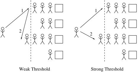
[image:15.612.190.423.72.193.2]Weak Threshold Strong Threshold 1
Figure 4: Weak and strong threshold models. A customer rechooses if and only if they would start behind the dashed line. In the weak model, the customer jumps to a second server, and may go to a longer line (2). In the strong model, the customer goes to the shorter of the two lines (1).
simple recurrence for thewi is easily solved and clearly increasing for suitably small δ. Hence, by taking a
δsmall enough, both sequences ofwi will be increasing.
Technically, we should choose a sequence of wi so that the the corresponding 8(0) =
P∞
i=1wi|i(0)|
is finite. We can easily modify the tail of thewi sequence above so that it is dominated by a geometrically
increasing sequence, where the ratio of successive terms is less than 1/λ. If we assume that in the initial
state sj(0)=0 for some j , thenjis eventually dominated by geometric series where the ratio of successive
terms is at mostλ. Hence we may find a suitable sequence ofwi such that
P∞
i=1wi|i(0)|is finite. From this it is clear that the conditions of Theorem 10 holds, proving the corollary.
For the closed model and the model with unaware customers, Theorems 8 and 10 do not immediately
apply. However, the technique of examining the terms in each i separately can still prove effective; for
example, it can be used to prove that the fixed point for the closed model given by the equations (4) is stable.
5
Threshold models
In practice, it may often be more efficient not to give all customers several choices, as each choice may have a corresponding cost (for example, a cost corresponding to communication). A threshold system reduces the number of choices by only allowing a customer a second random choice if the load at its first choice exceeds a fixed threshold. The customer begins by choosing a single queue uniformly at random: if the queue length at this first choice (excluding the incoming customer) is at most T , the customer queues there; otherwise, the customer chooses a second queue uniformly at random (with replacement). Two variations are now possible. In the weak threshold model, the customer waits at the second queue, regardless of whether it is longer or shorter than the first. In the strong threshold model, the customer queues at the shorter of its two choices. (See Figure 4.) One could also expand both models so that a customer has several successive choices, with a different threshold set for each choice, up to any fixed number of choices; here we model only the case where a customer has at most two choices. Although threshold systems have been shown to perform well in practice [7, 18, 35], our results distinguishing these two models are new.
5.1
Limiting systems
We consider the limiting system for the weak threshold model. The rate at which a queue changes size
depends on whether it has more or fewer than T customers. We first calculate dsi
pi = si −si+1 be the fraction of queues with exactly i customers. An arriving customer becomes the i th
customer in a queue if one of two events happen: either its first choice has i−1 customers, or its first choice
has T +1 or more customers and its second choice has i−1 customers. Hence over a time interval dt the
expected number of jumps from queues of size i−1 to i isλn(pi−1+sT+1pi−1). Similarly, the expected
number of jumps from queues of size i to i−1 is npidt. Hence we find
dsi
dt = λ(pi−1+sT+1pi−1)−pi ,i ≤T +1, or dsi
dt = λ(si−1−si)(1+sT+1)−(si−si+1) , i ≤T +1. (6)
The case where i ≥T +1 can be calculated similarly, yielding
dsi
dt = λ(si−1−si)sT+1−(si −si+1) , i >T +1. (7)
We now determine the fixed point. As usual, π0 = 1 and, because at the fixed point the rate at which
customers arrive must equal the rate at which they leave,π1=λ. In this case we also need to find the value
ofπT+1to be able to calculate further values ofπi. Using the fact that dsdti =0 at the fixed point yields that
for 2≤i≤ T +1,
πi =πi−1−λ(πi−2−πi−1)(1+πT+1). (8)
Recursively plugging in, we find
πT+1=1−
(1−λ)[((1+πT+1)λ)T+1−1]
(1+πT+1)λ−1 .
Given the threshold T ,πT+1can be computed effectively by finding the unique root between 0 and 1 of the
above equation. (The root is unique as the left hand side is increasing inπT+1, while the right hand side is
decreasing inπT+1.) Note that in this system the πi do not decrease doubly exponentially, although they
can decrease very quickly ifπT+1is sufficiently small.
The strong threshold model is given by the following differential equations:
dsi
dt = λ(si−1−si)(1+sT+1)−(si−si+1) , i≤ T +1; (9) dsi
dt = λ(s 2
i−1−s 2
i)−(si−si+1) , i >T +1. (10)
As equations (6) and (9) are the same, thre recurrence (8) also holds for the fixed point of the strong threshold system, soπT+1for the strong threshold system is calculated similarly.
For small thresholds, the behavior of this system is very similar to that of the supermarket system, as has been noted empirically previously in [7] and [35]. In fact, the strong threshold model is double exponentially decreasing.
Lemma 12 The fixed point for the strong threshold model decreases doubly exponentially.
Proof: To show that the fixed point decreases doubly exponentially, we note that it is sufficient to show that
πT+j+1 =λπT2+j for all j ≥ 1, from which the lemma follows by a simple induction. Moreover, to prove
that πT+j+1 = λπT2+j for all j ≥ 1, it is sufficient to show thatπT+2 = λπT2+1. That this is sufficient
follows from equation (10) and the fact that dsi
dt =0 at the fixed point, from which we obtain
λπ2
for i ≥T +2.
Hence, to prove the lemma, we now need only show thatπT+2=λπT2+1. From equation (9) we have
πT+2 = πT+1−λ(πT−πT+1)(1+πT+1),
which can be written in the form
πT+2−λπT2+1 = (1+λ)πT+1−λ(1+πT+1)πT. (11)
We show that the right hand side of equation (11) is 0. The recurrence (8) yields that
λ(πi−2−πi−1)(1+πT+1)=πi−1−πi.
Summing the left and right hand sides of the above equation for all values of i in the range 2≤ i ≤ T +1
yields
λ(1−πT)(1+πT+1)=λ−πT+1,
or more conveniently,
λ(1+πT+1)πT =(1+λ)πT+1.
Hence the right hand side of equation (11) is 0 and the lemma is proved.
5.2
Convergence and stability
For the strong threshold model, we can show that the infinite system converges exponentially to the fixed point, as we have done for the supermarket model. Unfortunately, for the weak threshold model, we have only been able to prove stability. We present both proofs here, beginning with the stability of the weak model.
It is convenient to write the derivatives di/dt obtained from equations (6) and (7) in the following form:
di
dt = λ(i−1−i)(1+πT+1)−(i−i+1)+λT+1(si−1−si) , i≤ T +1; (12) di
dt = λ(i−1−i)πT+1−(i −i+1)+λT+1(si−1−si) , i >T +1. (13)
Notice that we have made all the terms appear linear in i by leaving terms of the formλT+1(si−1−si) unexpanded.
Theorem 13 The fixed point of the weak threshold model is stable.
Proof: We shall assume thei are non-zero; the casei =0 can be handled as in Theorem 8. We examine the potential function given by the L1-distance D(t)=
P∞
i=1|i(t)|, and show that d Ddt ≤ 0. As in Theorem 8 we collect all terms with a factor ofi. For i 6= T +1, it is simple to verify that all terms are linear in i,
and that the coefficient of sum of all such terms is at most 0. For example, for i < T +1, the sum of the
terms ini is
(−λ(1+πT+1)−1)isgn(i)+λ(1+πT+1)isgn(i+1)+isgn(i−1),
The only difficulty arises in theT+1 term. Note the different form of the first expression on the right
hand side of (12) and (13) : one has a factor ofπT+1, and one has a factor of 1+πT+1. Hence, in gathering
the terms inT+1, we have the following sum:
(−λ(1+πT+1)−1)T+1sgn(T+1)+λπT+1T+1sgn(T+2)
+T+1sgn(T)+T+1
∞ X
j=1
λ(sj−1−sj)sgn(j).
Let us suppose that T, T+1, andT+2 are all strictly positive; all other cases are similar. Then the
above summation reduces to
−λT+1+T+1
∞ X
j=1
λ(sj−1−sj)sgn(j).
The largest value the second expression can take is when sgn(j) = 1 for all j , in which case it isλT+1.
Hence, regardless of the signs of the remainingi, we find that the coefficient of the sum of the terms in
T+1is also at most 0.
For the weak threshold model, proving convergence to the fixed point appears possible using the tech-nique of [33], although their methods do not appear to provide bounds on the rate of covergence. (Note that stability does not imply convergence, nor does convergence imply our strong notion of stability, namely that the L1distance is non-increasing.)
We can, however, show that the strong threshold model does converge exponentially. As in Theorem 13, it will help us to rewrite the derivatives di
dt for the infinite system of the strong threshold model obtained
from the equations (9) and (10) in the following form:
di
dt = λ(i−1−i)(1+πT+1)−(i−i+1)+λT+1(si−1−si) , i≤ T +1; (14) di
dt = λ( 2
i−1+2πi−1i−1−i2−2πii)−(i−i+1) , i >T +1. (15) Theorem 14 The strong threshold model converges exponentially to its fixed point from any initial state where there exists a k such that sk(0)=0.
Proof: We shall find an increasing sequence wi and δ > 0 such that for 8(t) = P
iwi|i(t)|, we have
d8/dt = −δ8. As in Theorem 10, the proof will depend on finding a sequencewi such that the terms of
d8/dt ini sum to at most−δwi|i|. In fact, any sequence satisfying
wi+1 ≤ wi+ wi(
1−δ)−wi−1
λ(1+πT+1)
, i <T +1 (16)
wi+1 ≤ wi+ wi(
1−δ)−wi−1
λ(1+2πi)
, i ≥T +1 (17)
will suffice, and it is easy to verify that such sequences exist, as in Theorem 10. That this condition suffices
can be easily checked by grouping all thei terms from equations (14) and (15) for alli exceptT+1. The
difficulty for theT+1terms lies in the extraneousλT+1(si−1−si)terms in equation (14).
We now bound the sum of the terms inT+1. We consider here only the case where alli are positive;
other cases are similar. The sum of all the terms inT+1is
(−λ(1+πT+1)−1)wT+1T+1sgn(T+1)+λ(2πT+1+T+1)wT+2T+1sgn(T+2)+
wTT+1sgn(T)+T+1
T+1
X
j=1
If alli are positive this reduces to
(−λ(1+πT+1)−1)wT+1T+1+λ(2πT+1+T+1)wT+2T+1+wTT+1+T+1
T+1
X
j=1
wjλ(sj−1−sj).
As thewi are increasing, the termT+1
PT+1
j=1 wjλ(sj−1−sj)can be bounded above by
T+1
T+1
X
j=1
wT+1λ(sj−1−sj)=T+1wT+1λ(1−πT+1−T+1).
Hence the sum of the terms inT+1is bounded above by
(−λ(2πT+1+T+1)−1)wT+1T+1+λ(2πT+1+T+1)wT+2T+1+wTT+1,
and it is easily checked that equation (17) is sufficient to guarantee that this sum is at most−δwT+1T+1.
Finally, we note that we may choose the wi so that they are eventually dominated by a geometric
se-ries, as in Theorem 10. Since the tail of the fixed point for the strong threshold model decreases doubly exponentially by Lemma 12, we have
8(0)= ∞ X
i=1
wi|i| = k X
i=1
wi|i| + ∞ X
i=k wiπi
is finite.
5.3
Simulations of threshold schemes
We first demonstrate the accuracy of the differential equations in describing system behavior. We consider the weak threshold scheme of Section 5 (where customers who make a second choice always queue at their second choice) with 100 queues at various arrival rates in Table 2. As before, simulations were done for 100,000 units of time with the first 10,000 thrown out for calculation purposes. For arrival rates up to 95% of the service rate, the predictions are within approximately 2% of the simulation results; with smaller arrival rates, the prediction is even more accurate. These results again demonstrates the accuracy of this approach. We also compare the strong threshold scheme and the weak threshold scheme to the standard super-market model where each customer always has two choices. Since the performance of the weak threshold scheme depends on the threshold chosen, we graph the best choice and second best choice for specific
ar-rival ratesλ. (Note the strong threshold scheme with the threshold set to 0 is equivalent to the supermarket
model.) As one might expect, threshold schemes do not perform as well as the supermarket model (See Figure 5). It is worth noting, however, that even the weak threshold scheme performs almost as well for reasonable arrival rates (sayλ < 0.9), despite the proven difference in the behavior of the tails (exponen-tial versus doubly exponen(exponen-tial dropoff). In many applications threshold schemes may be suitable, or even preferable, because they reduce the overall amount of communication that is necessary. Even though the threshold must be chosen appropriately to match the load, small thresholds are adequate over a large range of arrival rates.
6
Concluding remarks
λ Threshold Simulation Prediction Relative Error (%)
0.50 0 1.3360 1.3333 0.2025
1 1.4457 1.4444 0.0900
0.70 0 1.9635 1.9608 0.1377
1 1.8144 1.8074 0.3873
2 2.0150 2.0109 0.2039
0.80 0 2.7868 2.7778 0.3240
1 2.2493 2.2346 0.6578
2 2.3518 2.3387 0.5601
0.90 1 3.5322 3.4931 1.1194
2 3.1497 3.1067 1.3841
3 3.2903 3.2580 0.9914
0.95 2 4.5767 4.4464 2.9305
3 4.2434 4.1274 2.8105
4 4.3929 4.3061 2.0158
0.99 4 8.1969 7.4323 10.2875
5 7.5253 6.8674 9.5800
[image:20.612.157.454.95.352.2]6 7.6375 6.9369 10.0996
Table 2: Simulations versus estimates for the weak threshold model: 100 queues.
0 1 2 3 4 5
0 . 5 0 . 6 0 . 7 0 . 8 0 . 9 1
Arrival Rate
Average Time
[image:20.612.106.500.431.654.2]2 choices Strong, T=1 Weak, best Weak, 2nd best
to the supermarket model and several variations, including the case of fixed service times and threshold systems. Besides allowing an analysis of these systems, our work demonstrates that there are important behavioral differences between systems where customers have one choice and systems where they have more than one choice. In particular, we have shown that using two choices can lead to an exponential improvement in the expected time in the system over using one choice; using more choices leads to much less substantial improvements.
Extrapolating from our results, we believe that the paradigm of using load information from a small random sample of possible destinations will prove effective in many load balancing scenarios. Indeed, the effectiveness of this general approach has been noted recently in practical load balancing scenarios [30] as well as for load profiling in real-time systems [6].
Although our methodology has been successful for several models, there remain several open questions. We conjecture that the closed model and the weak threshold model converge exponentially, although a proof appears to require different techniques than given here. The problem of analyzing the behavior of these simple randomized strategies on small systems and systems with fixed network topologies also appears to lie outside the range of our techniques. Finally, it would be interesting to test the performance of these methods in the context of more complex service and arrival distributions, such as heavy-tailed distributions.
References
[1] I. J. B. F. Adan, G. van Houtum, and J. van der Wal. Upper and lower bounds for the waiting time in the symmetric shortest queue system. Annals of Operations Research, 48:197–217, 1994.
[2] I. J. B. F. Adan, J. Wessels, and W. H. M. Zijm. Analysis of the symmetric shortest queue problem.
Stochastic Models, 6:691–713, 1990.
[3] I. J. B. F. Adan, J. Wessels, and W. H. M. Zijm. Analysis of the asymmetric shortest queue problem.
Queueing Systems, 8:1–58, 1991.
[4] M. Alanyali and B. Hajek. Analysis of simple algorithms for dynamic load balancing. In INFOCOM
’95, 1995. To appear in Math. Oper. Res.
[5] Y. Azar, A. Broder, A. Karlin, and E. Upfal. Balanced allocations. In Proceedings of the 26th ACM
Symposium on the Theory of Computing, pages 593–602, 1994.
[6] A. Bestavros. Load profiling: A methodology for scheduling real-time tasks in a distributed system. In Proceedings of ICDCS’97: The IEEE International Conference on Distributed Computing Systems, 1997.
[7] D. L. Eager, E. D. Lazokwska, and J. Zahorjan. Adaptive load sharing in homogeneous distributed systems. IEEE Transactions on Software Engineering, 12:662–675, 1986.
[8] D. L. Eager, E. D. Lazokwska, and J. Zahorjan. A comparison of receiver-initiated and sender-initiated adaptive load sharing. Performance Evaluation Review, 16:53–68, March 1986.
[9] D. L. Eager, E. D. Lazokwska, and J. Zahorjan. The limited performance benefits of migrating active processes for load sharing. Performance Evaluation Review, 16:63–72, May 1988. Special Issue on the 1988 SIGMETRICS Conference.
[11] B. Hajek. Asymptotic analysis of an assignment problem arising in a distributed communications protocol. In Proceedings of the 27th Conference on Decision and Control, pages 1455–1459, 1988.
[12] M. Harchol-Balter and D. Wolfe. Bounding delays in packet-routing networks. In Proceedings of the
Twenty-Seventh Annual ACM Symposium on the Theory of Computing, pages 248–257, 1995.
[13] R. M. Karp, M. Luby, and F. Meyer auf der Heide. Efficient PRAM simulation on a distributed memory machine. In Proceedings of the 24th ACM Symposium on the Theory of Computing, pages 318–326, 1992.
[14] R. M. Karp and M. Sipser. Maximum matchings in sparse random graphs. In Proceedings of the 22nd
IEEE Symposium on Foundations of Computer Science, pages 364–375, 1981.
[15] R. M. Karp, U. V. Vazirani, and V. V. Vazirani. An optimal algorithm for on-line bipartite matching. In Proceedings of the 22nd ACM Symposium on the Theory of Computing, pages 352–358, 1990.
[16] F. P. Kelly. Reversibility and Stochastic Networks. John Wiley and Sons, 1979.
[17] L. Kleinrock. Queueing Systems, Volume I: Theory. John Wiley and Sons, 1976.
[18] T. Kunz. The influence of different workload descriptions on a heuristic load balancing scheme. IEEE
Transactions on Software Engineering, 17:725–730, 1991.
[19] T. G. Kurtz. Solutions of ordinary differential equations as limits of pure jump Markov processes.
Journal of Applied Probability, 7:49–58, 1970.
[20] T. G. Kurtz. Limit theorems for sequences of jump Markov processes approximating ordinary differ-ential processes. Journal of Applied Probability, 8:344–356, 1971.
[21] T. G. Kurtz. Strong approximation theorems for density dependent Markov chains. Stochastic
Pro-cesses and Applications, 6:223–240, 1978.
[22] T. G. Kurtz. Approximation of Population Processes. CBMS-NSF Regional Conf. Series in Applied
Math. SIAM, 1981.
[23] A. N. Michel and R. K. Miller. Qualitative Analysis of Large Scale Dynamical Systems. Academic Press, Inc., 1977.
[24] M. Mitzenmacher. How useful is old information? Submitted to PODC ’97.
[25] M. Mitzenmacher. Bounds on the greedy routing algorithm for array networks. In Proceedings of the
Sixth Annual ACM Symposium on Parallel Algorithms and Architectures, pages 248–259, 1994. To
appear in the Journal of Computer Systems and Science.
[26] M. Mitzenmacher. Constant time per edge is optimal on rooted tree networks. In Proceedings of the
Eighth Annual ACM Symposium on Parallel Algorithms and Architectures, pages 162–169, 1996.
[27] M. Mitzenmacher. Density dependent jump Markov processes and applications to load balancing. In
Proceedings of the 37th IEEE Symposium on Foundations of Computer Science, pages 213–222, 1996.
[29] R. Righter. and J. Shanthikumar. Extremal properties of the FIFO discipline in queueing networks.
Journal of Applied Probability, 29:967–978, November 1992.
[30] J. R. Santos and R. Muntz. Design of the RIO (Randomized I/O) storage server. Computer science division, University of California, Los Angeles, May 1997.
[31] A. Shwartz and A. Weiss. Large Deviations for Performance Analysis. Chapman & Hall, 1995.
[32] G. D. Stamoulis and J. N. Tsitsiklis. The efficiency of greedy routing in hypercubes and butterflies.
IEEE Transactions on Communications, 42(11):3051–3061, November 1994. An early version
ap-peared in the Proceedings of the Second Annual ACM Symposium on Parallel Algorithms and
Archi-tectures, p. 248-259, 1991.
[33] N. D. Vvedenskaya, R. L. Dobrushin, and F. I. Karpelevich. Queueing system with selection of the shortest of two queues: An asymptotic approach. Problems of Information Transmission, 32:15–27, 1996.
[34] N. C. Wormald. Differential equations for random processes and random graphs. Annals of Appl.
Prob., 17:1217–1235, 1995.
[35] S. Zhou. A trace-driven simulation study of dynamic load balancing. IEEE Transactions on Software
Engineering, 14:1327–1341, 1988.
A
From infinite to finite: Kurtz’s theorem
In this section, we briefly describe the formal theory that connects the limiting system with systems of finite size, based on the work of Kurtz. As even stating an appropriate theorem requires a great deal of background and notation, we here provide only an informal argument; further explication with regard to load balancing problems is available in [28] or [33]; more general works covering the appropriat theory include [10, 31]. The supermarket model is an example of a density dependent family of jump Markov processes. Informally, such a family is a one parameter family of Markov processes, where the parameter n corresponds to the total population size (or, in some cases, area or volume). The states can be normalized and interpreted as measuring population densities, so that the transition rates depend only on these densities. As we have seen in Section 2.1, for the supermarket model the transition rates between states depend only upon the
densities si. Hence the supermarket model fits our informal definition of a density dependent family. The
limiting system corresponding to a density dependent family is the limiting model as the population size grows arbitrarily large.
Kurtz’s work provides a basis for relating the limiting system for a density dependent family to the corresponding finite systems. Essentially, Kurtz’s theorem provides a law of large numbers and Chernoff-like bounds for density dependent families. The primary differences between the limiting system and the finite system are:
• The limiting system is deterministic; the finite system is random.
• The limiting system is continuous; the finite system has jump sizes that are discrete values.
Imagine starting both systems from the same point for a small period of time. Since the jump rates for both processes are initially the same, they will have nearly the same behavior. Now suppose that if two points are close in the infinite dimensional space then their transition rates are also close; this is called the