Binary Periodic Synchronizing
Sequences
Marcin Skubiszewski
This article will also appear in Theoretical Computer Science, Part A, Volume 99 (October 1992).
Author’s electronic address: [email protected]
c
Digital Equipment Corporation 1991
In this article, we consider words overf0;1g. The autodistance of such a word is the lowest among the Hamming distances between the word and its images by circular permutations other than identity; the word’s reverse autodistance is the highest among these distances. For each l2, we study the words of lengthlwhose autodistance and reverse autodistance are close to l =2 (we call such words synchronizing sequences).
We establish, for everyl3, an upper bound on the autodistance of words of lengthl. This upper bound, called up (l), is very close tol =2.
We briefly describe the maximal period linear recurring sequences, a previously known family of words over f0;1g; such words exist for every length of the form l = 2
n
1 and their autodistances achieve the upper bound up (l).
Examples of words whose autodistance and reverse autodistance are both equal or close to up (l) are discussed; we describe the method (based on simulated annealing) which was used to find the examples.
We prove that, for sufficiently largel, an arbitrarily high proportion of words of lengthl will have both their autodistance and reverse autodistance very close to up (l).
R ´esum ´e
Nous consid´erons dans cet article des mots sur f0;1g. Nous appelons autodistance d’un tel mot la plus petite des distances de Hamming entre lui-mˆeme et ses images par des permutations circulaires non identiques; l’autodistance inverse du mot d´esigne la plus grande de ces distances. Pour toutl2, nous ´etudions les mots de longueurldont l’autodistance et l’autodistance inverse sont toutes les deux proches del =2 (de tels mots seront appel´es suites synchronisantes).
Pour toutl3, nous ´etablissons une borne sup´erieure sur l’autodistance des mots de longueur l. Cette borne sup´erieure, not´ee up (l), est tr`es proche del =2.
Nous pr´esentons bri`evement les suites lin´eairement r´ecurrentes de p´eriode maximale, une famille d´ej`a ´etudi´ee de mots sur f0;1g; de tels mots existent pour toute longueur de forme l= 2
n
1 et leur autodistance atteint la borne up (l).
Nous consid´erons des exemples de mots dont l’autodistance et l’autodistance inverse sont toutes les deux proches de up (l) ou ´egales `a cette valeur; nous d´ecrivons la m´ethode (une adaptation du recuit simul´e) qui a permis de trouver ces exemples.
1.1 Subject of the article : : : : : : : : : : : : : : : : : : : : : : : : : : : : 1 1.2 Contents : : : : : : : : : : : : : : : : : : : : : : : : : : : : : : : : : : 1
2 Definitions and Notation 2
2.1 Basic notation : : : : : : : : : : : : : : : : : : : : : : : : : : : : : : : 2 2.2 Notation of objects defined in the article : : : : : : : : : : : : : : : : : 2 2.3 Autodistance and synchronizing sequences : : : : : : : : : : : : : : 2
3 Bounds on Synchronizing Sequence Characteristics 4
3.1 An upper bound on the autodistance : : : : : : : : : : : : : : : : : : : 4 3.2 Non existence of certain uniform sequences : : : : : : : : : : : : : : 7 3.3 Uniformity of certain sequences : : : : : : : : : : : : : : : : : : : : : 9
4 Maximal Period Linear Recurring Sequences 9
5 Example Double Synchronizing Sequences 10
5.1 How the examples have been found : : : : : : : : : : : : : : : : : : : 10 5.2 What we can learn from the examples : : : : : : : : : : : : : : : : : : 11 5.2.1 The autodistance : : : : : : : : : : : : : : : : : : : : : : : : : : 11 5.2.2 The reverse autodistance of optimal synchronizing sequences : : : 14
6 Double Synchronizing Sequences of Lengthl !+∞ 14
6.1 The result : : : : : : : : : : : : : : : : : : : : : : : : : : : : : : : : : : 14 6.2 How the proof is organized : : : : : : : : : : : : : : : : : : : : : : : : 14 6.3 The two capital lemmas : : : : : : : : : : : : : : : : : : : : : : : : : : 15 6.4 Conventions : : : : : : : : : : : : : : : : : : : : : : : : : : : : : : : : 15 6.5 Auxiliary lemmas : : : : : : : : : : : : : : : : : : : : : : : : : : : : : : 16 6.6 The setsE
p;D
: : : : : : : : : : : : : : : : : : : : : : : : : : : : : : : 17 6.7 More auxiliary lemmas : : : : : : : : : : : : : : : : : : : : : : : : : : 19 6.8 The setsD
d;p
: : : : : : : : : : : : : : : : : : : : : : : : : : : : : : : : 20 6.9 Conclusion : : : : : : : : : : : : : : : : : : : : : : : : : : : : : : : : : 26 6.10 The proof of Capital Lemma 2 : : : : : : : : : : : : : : : : : : : : : : 26
1 Introduction
1.1 Subject of the article
Modern radio techniques, including radar and spread-spectrum communications, make use of finite sequences of bits exhibiting various correlation properties (e.g. [5], [2] chapters 10 and 12, [1]). The correlation properties of a sequence measure how easily it can be distinguished, after a transmission with errors, from other related sequences (the notion of related sequences is application-dependent).
We study here two correlation properties, the autodistance and the reverse autodistance. The autodistance measures how well, in the worst case, the receiver will be able to distinguish between the sequence and a non-identical circular permutation of it (in this case, we consider that circular permutations of a sequence are related to it). The reverse autodistance measures the difficulty that the receiver will have, in the worst case, distinguishing between the sequence and a circular permutation of its one’s complement (here, we consider that circular permutations of the one’s complement of a sequence are related to the sequence).
In this study, we focus on searching for, and estimating the number of, sequences that exhibit a high autodistance (the synchronizing sequences) and those that exhibit both a high autodistance and a low reverse autodistance (the double synchronizing sequences).
1.2 Contents
Section 2 of the article introduces the necessary notation and mathematical objects (including precise definitions of autodistance and reverse autodistance).
In Section 3, we investigate which values the autodistance and reverse autodistance can attain. We establish, for each lengthl, an upper bound on the autodistance of sequences of this length (Section 3.1); we complete this basic result with several remarks about the reverse autodistance of certain classes of sequences (Sections 3.2–3.3).
In Sections 4-6, we either find, or prove the existence of, sequences whose autodistance and reverse autodistance approach the previously established bounds.
In Section 4, quoting already known results [4], we introduce the maximal period linear recurring sequences, a family of double synchronizing sequences which achieve the bounds for certain lengthsl.
In Section 5, we describe examples of double synchronizing sequences whose lengths are between 3 and 405; these examples achieve, or almost achieve, the bounds. We present a computational method, based on simulated annealing, which we used to find the examples.
2 Definitions and Notation 2.1 Basic notation
iuj greatest common divisor (GCD) ofi;j∈N [a::b] interval
n
i∈Z aib o
[a::b) interval n
i∈Z ai<b o
N2+ set of natural numbers2 f0;1g
2+
set of words overf0;1gof length2 f0;1g
l
forl∈N2+, set of words overf0;1gof lengthl jSj jEj length of the wordS∈f0;1g
2+
; cardinality of the setE jSj
0 jSj
1 number of zeros (resp. ones) inS∈f0;1g
2+
(F x)
x∈X the family of elements F
x, indexed by elements
x∈X; by definition,j(F x)
x∈X j=jXj jFj
A
number of elements of the familyF belonging to the setA; ifF = (F x)
x∈X, then
jFj A
= n
x∈X F
x ∈ A
o
A4B symmetrical difference between sets:A4B = (A[B) (A\B) xA forx∈R andAR, the set
n
xy y∈A
o
; the definitions of A+xandA xare analogous
S[i] forS∈f0;1g
2+and 0
i<jSj, thei-th digit ofS
p circular permutation by
pof words fromf0;1g
2+:
p(
S)[i] = S
(i+p) modjSj
d (S;T) forS;T ∈f0;1g l
, the Hamming distance betweenSandT:
d (S;T) = n
i∈[0::l) S[i] ≠ T[i] o
2.2 Notation of objects defined in the article
d (S) forS∈f0;1g
2+
, the autodistance ofS (Definition 1 below) d0
(S) forS∈f0;1g
2+
, the reverse autodistance ofS(Definition 2 below) up (l) forl∈N;l3, up (l) = 2b(l+ 1)=4c(Definition 7 below)
2.3 Autodistance and synchronizing sequences
Definition 1 (autodistance) For S ∈ f0;1g
2+, the autodistance of
S is the minimum of the Hamming distances betweenSand all its images by circular permutations other than identity:
d (S) = min p∈[1::jSj)
d S; p(
Definition 2 (reverse autodistance) ForS ∈ f0;1g
2+
, the reverse autodistance ofS is the maximum of the Hamming distances betweenSand all its images by circular permutations:
d0
(S) = max p∈[0::jSj)
d S; p(
S)
Examples: The null word of any length satisfies d (S) = d 0
(S) = 0. The words 001and 0011satisfy
d (001) = d0
(001) = 2 d (0011) = 2 d0
(0011) = 4
Definition 3 (optimal synchronizing sequence) An optimal synchronizing sequence of length
l ∈N2+ is a wordS ∈f0;1g l
whose autodistance is maximal; in symbols,S ∈f0;1g l
is an optimal synchronizing sequence if and only if
∀(T ∈f0;1g l
) d (T)d (S)
Informally, we call any wordS ∈f0;1g l
whose autodistance is maximal or nearly maximal a synchronizing sequence of lengthl.
Definition 4 (double-optimal synchronizing sequence) A double-optimal synchronizing se-quence of lengthl ∈N2+ is a wordS ∈ f0;1g
l
whose autodistance is maximal, and whose reverse autodistance is minimal among all words inf0;1g
l
having the maximal autodistance; in symbols,S∈f0;1g
l
is a double-optimal synchronizing sequence if and only if
∀(T ∈f0;1g l
) d (T)<d (S)∨ d (T) = d (S)∧d 0
(T)d 0
(S)
Informally, any wordS ∈ f0;1g l
whose autodistance is maximal or nearly maximal and whose reverse autodistance is, among the words having the same autodistance asS, minimal or nearly minimal, will be called a double synchronizing sequence of lengthl.
Definition 5 (uniform sequence) A uniform sequence is a wordS∈f0;1g
2+
such that
d (S) = d 0
(S)
It follows from Definitions 1 and 2 above that the sequence S ∈ f0;1g
2+ is uniform if
and only if the number d (S;(S)), where is a non-identical circular permutation, does not depend on the choice of.
Definition 6 (uniform optimal synchronizing sequence) A word fromf0;1g
2+
is a uniform optimal synchronizing sequence if it is a uniform sequence and an optimal synchronizing sequence.
Informally, any word fromf0;1g
2+ which is both a uniform sequence and a synchronizing
sequence will be called a uniform synchronizing sequence.
It follows from the definitions above that a uniform optimal synchronizing sequence is also a double-optimal synchronizing sequence.
Example: The word 001 is a uniform optimal synchronizing sequence. Long optimal synchronizing sequences are never trivial.
3 Bounds on Synchronizing Sequence Characteristics
Theorem 1 below establishes an upper bound on the autodistances of synchronizing sequences. Theorems 2 and 3 establish that uniform synchronizing sequences of certain forms do not exist. Theorem 4 states that all optimal synchronizing sequences in a certain category are uniform.
3.1 An upper bound on the autodistance
Theorem 1 (an upper bound on the autodistance) For everyl∈N;l3, the autodistance of every wordS ∈f0;1g
l
is less than or equal to the value given in the following table (for
n∈Z):
l=jSj d (S) 4n 2n 4n+ 1 2n 4n+ 2 2n 4n+ 3 2n+ 2
Definition 7 (up (l)) For everyl3, the upper bound given in the table in Theorem 1 will be denoted up (l).
In order to prove the theorem, let us establish two lemmas.
Lemma 1 (parity of d (S)) The autodistance of every wordS∈f0;1g
2+is even.
Proof: By Definition 1, for some p ∈ N we have d (S) = d S; p(
S)
. It is therefore sufficient to prove that the Hamming distance between a wordS ∈ f0;1g
2+
LetT be a circular permutation ofS. We define, forx;y∈f0;1g, the four sets A xy = n i∈ 0:: jSj
S[i] =x∧T[i] =y o
which trivially have the following properties:
jSj
1 = jA10j+jA11j
jTj
1 = jA01j+jA11j
d (S;T) = jA01j+jA10j These equations, together with the fact thatjSj
1=jTj
1, imply
d (S;T) = 2jA01j
so d (S;T) is even. 2
Lemma 2 (a weaker version of Theorem 1) For l 3, the autodistance of every word S ∈f0;1g
l
is less than or equal todl =2e.
Proof: LetS∈f0;1g l
. We define fori∈[0::l) andx∈f0;1g:
N x[
i] = n
p∈[0::l) p(
S)[i] =x o
By definition of
p( S),
N x[
i] = n
p∈[0::l) S[(i+p) modl] =x o
and, regardless ofi,
N x[
i] =jSj
x (1)
Let us define the total autodistance ofS, calledK, as
K= l 1 X p=0 d S; p( S) (2)
By definition of d (S;T),Ksatisfies:
K = l 1 X p=0 n
i∈[0::l) S[i] ≠ p(
S)[i] o = n
(p;i)∈[0::l)
2
S[i] ≠ p(
S)[i] o = l 1 X i=0 n
p∈[0::l) S[i] ≠ p(
S)[i] o
= X
i∈[0::l) S[i]=0
N1[i] + X
i∈[0::l) S[i]=1
N0[i]
= X
i∈[0::l) S[i]=0
jSj
1+
X
i∈[0::l) S[i]=1
jSj
0 (by (1))
K = 2jSj
0jSj
The autodistance ofS is, by its definition, the minimum of the family d S; p(
S)
p∈[1::l) . Let us define the average autodistance ofS, calledM, as the average of the same family:
M =
P l 1 p=1
d S; p(
S)
l 1
(4)
This definition implies thatM d (S).
Equations (2) and (4) and the fact that d (S;0(S)) = 0, lead to the following expression ofM:
M =
K
l 1
M =
2jSj
0jSj
1
l 1
(by (3)) (5)
Iflis even, M is maximal forjSj
0 =jSj
1 =l =2, and we have,
M
2(l =2)(l =2)
l 1
M
l 2 +
1 2(1 1=l) Sincel3,
M < l 2+ 1 Since d (S)M and d (S)∈Z,
d (S) l 2 and the lemma holds forleven.
Iflis odd, M is maximal forjSj
0= (l 1)=2 andjSj
1= (l+ 1)=2. We have therefore,
M
2(l =2 + 1=2)(l =2 1=2)
l 1
M
l+ 1
2 (6)
Then,
d (S)dl =2e
and the lemma holds forlodd. 2
Proof of Theorem 1: Lemma 2 implies that, forl3, no word can have an autodistance greater than the value d (S) listed in the table below:
Lemma 1 says that no word can have an autodistance of the form 2n+ 1, which makes us
deduce the table in Theorem 1 from the one above. 2
3.2 Non existence of certain uniform sequences
Lemma 3 (domain of d0
(S)) For any wordS∈f0;1g l
;l∈N2+, the reverse autodistance of S is even and satisfies
d (S)d 0
(S)l (7)
Proof: Substituting d0
(S) for d (S) in the proof of Lemma 1 gives the evenness of d 0
(S). Relation (7) results directly from the definitions of autodistance and reverse autodistance. 2
Theorem 2 (nontrivial uniform sequences forl 1 prime) Let l ∈ N2+ and let l 1 be prime. Then among the wordsS ∈f0;1g
l
, exactly those verifying one of the conditions
jSj
0 = 0 (8)
jSj
0 = 1 (9)
jSj
0 = l (10)
jSj
0 = l 1 (11)
are uniform sequences.
Proof: The reader may easily verify the fact that each of the conditions (8)–(11) implies thatSis a uniform sequence.
Supposing thatl 1 is prime and thatS ∈f0;1g l
is a uniform sequence, let us prove that one of relations (8)–(11) holds. From the definitions of autodistance and reverse autodistance, we get
∀(p∈[1::l)) d (S)d S; p(
S)
d
0 (S)
which implies that M, the average autodistance of S defined as in the proof of Lemma 2, relation (4), satisfies
d (S)M d 0
(S) Since d (S) = d
0
(S), we successively get
M = d (S)
M ∈ 2N (from Lemma (1)) 2jSj
0jSj
1
l 1
∈ 2N (from (5))
jSj
0(1 jSj
0) ∈ (l 1)N
jSj
0 ∈ (l 1)N or (1 jSj
Theorem 3 (uniform optimal synchronizing sequences) Letl∈N2+. If one of the following holds
i. l= 4nwheren∈N and p
n∉N. ii. l= 4n+ 1 wheren∈N and
p
8n+ 1∉N. iii. l= 4n+ 2 wheren∈N and
p
3n+ 1∉N.
then no uniform sequenceS ∈f0;1g l
will satisfy the equality d (S) = up (l).
Proof: Suppose thatS ∈f0;1g l
is a uniform sequence with d (S) = d 0
(S) = up (l). Then, reasoning as in the proof of Theorem 2, we can say thatM, the average autodistance ofS, satisfies
M = d (S) which, by (5), translates into
2jSj
0(l jSj
0) = (l 1)up (l) (13)
If (i) holds, thenl= 4n, and (13) becomes
jSj
2
0 4njSj
0+ 4n
2
n= 0 Solving this second degree equation injSj
0, we deduce that (13) is equivalent to
jSj
0= 2n+
p
n or jSj
0= 2n
p n which is impossible sincep
n∉N. If (ii) holds, then (13) becomes
jSj
2
0 (4n+ 1)jSj
0+ 4n
2 = 0
jSj
0=
1 2
4n+ 1 + p
8n+ 1
or jSj
0=
1 2
4n+ 1
p 8n+ 1
(14)
Recalling that the square root of a natural number is either natural or irrational, we deduce that
p
8n+ 1 is irrational. Therefore, the alternative (14) implies thatjSj
0 is
irrational, which is impossible. If (iii) holds, then (13) becomes
jSj
2
0 2(2n+ 1)jSj
0+ (4n+ 1)n = 0
jSj
0= 2n+ 1 + p
3n+ 1 or jSj
0 = 2n+ 1
p
3n+ 1 (15)
which is impossible since p
3.3 Uniformity of certain sequences
Theorem 4 (certain sequences are uniform) Forl= 4n+ 3;n∈N, every word fromf0;1g l whose autodistance is equal to up (l), is a uniform optimal synchronizing sequence.
Theorem 5 below says that sequences satisfying the hypotheses of Theorem 4 exist for l = 2
n
1;n∈N2+. In Section 5.2 (Figure 2 and Table 1) examples of sequences are quoted forl= 3;7;11;15;19;23;31;35.
Proof of Theorem 4: LetSsatisfy the hypotheses of the theorem. ThenSis, by Theorem 1 and by the definition of up (l), an optimal synchronizing sequence.
Let us prove thatSis a uniform sequence. We useM, as defined by equation (4) in the proof of Lemma 2. Sincelis odd, we can, as in the proof of Lemma 2, obtain inequality (6). This inequality and the fact that d (S) =
l+1
2 imply thatM d (S). SinceM is, by its definition, greater than or equal to d (S), we get
M = d (S)
The average and the minimum of the finite family of integers d S; p(
S)
p∈[1::l)
are then equal. All the numbers in the family are therefore equal and d0
(S) = d (S). 2
4 Maximal Period Linear Recurring Sequences Theorem 5 (up (l) is optimal forl= 2
n
1) For every l of the forml = 2 n
1;n ∈ N2+, there exists a wordS
n∈ f0;1g
l
verifying
d (S n) = d
0 (S
n) = up (
l) (16)
Since this theorem is a straightforward corollary of known results, we will not quote the proof in its entirety. Instead, we only describe a way to construct the sequence S
n. The proof that this construction is correct and that the resultingS
nsatisfies relation (16) is a direct consequence of well-known results from the theory of finite fields (see e.g. [4], paragraphs 2.11, 6.32, 6.33 and 7.44). The construction itself is discussed in detail by Sarwate and Pursley ([7], Section 3).
Construction: Let GF2 denote the Galois field of order 2 (i.e. the field composed of
elements 0 and 1) and GF2[X] denote the ring of polynomials over GF2.
For everyn ∈N2+, there exists in GF2[X] at least one primitive polynomial of degreen (see [4], 2.11). Let us choose one such polynomial and call itP
n; the coefficients of P
n will be calledp0;;p
n(with p
n= 1):
P n(
X) =p0+p1X++p n
P
ncan be used as the characteristic polynomial to build an infinite linear feedback sequence of bitsS
0
n. To build S
0
n, we arbitrarily choose its first
nbitsS 0 n[0]
;. . .;S 0 n[
n 1], with the only restriction that these bits may not be all equal to 0 (this gives us 2n
1 different choices ofS
0 n
). Then, we define the other bits ofS 0 n
by the recurrence formula
0 =p0S 0 n[
i] +p1S 0 n[
i+ 1] ++p n
S 0 n[
i+n] (for anyi∈N) (17) which translates into
S 0 n[
i+n] =p0S 0 n[
i] +p1S 0 n[
i+ 1] ++p n 1
S 0 n[
i+n 1] (for anyi∈N) (18)
The sequenceS 0
nis periodic and its least period is l= 2
n
1 (see [4], 6.33). We defineS nto be the left factor ofS
0
nof length
l(thereforeS
nrepresents one period of S
0 n).
S
nsatisfies (16) (see [4], 7.44).
Consequences of the theorem: Theorem 5 implies that for all valueslof the form 2 n
1, the upper bound up (l) is achieved by some word fromf0;1g
l
. For these values oflthe upper bound up (l) can therefore not be improved.
The results presented in the remainder of this article imply that, in fact, the upper bound up (l) is optimal or nearly optimal for any lengthl.
5 Example Double Synchronizing Sequences 5.1 How the examples have been found
Simulated annealing, the technique used here to find double synchronizing sequences, was first described by Kirkpatrick et al. [3]. Let us describe briefly both the technique and the way in which it has been adapted to our problem.
Simulated annealing is an optimization algorithm. It provides approximate solutions to difficult problems (i.e. to problems for which finding the global optimum would involve an extremely long computing time). More precisely, for a setX, on which is defined a function, called energy,E : X ! R, simulated annealing will try to find an elementx ∈X such that E(x) be as low as possible.
In our case, the algorithm is run separately for each value ofland we haveX =f0;1g l
. When searching for synchronizing sequences, we try to maximize d (x); therefore E(x) = d (x). When searching for double synchronizing sequences, we try both to maximize d (x) and to minimize d0
(x). In this case, the choice ofE is not obvious; after experimentation, the author chose E(x) = d
0
(x) 3d (x), although various other formulas apparently lead to identical results.
E(x) E(y). In our case, we consider that two words from f0;1g l
are neighbors if their Hamming distance is equal to 0 or 1. For the two energy functions mentionned above, this implies that ify∈N(x), then respectivelyjE(x) E(y)j2 orjE(x) E(y)j8.
The simulated annealing algorithm is a loop composed of a high number of similar steps. In each step, the algorithm tries to update the current solutionx∈X. To do so, it randomly chooses a solution y ∈ N(x). Then, if y is better thanx (i.e. E(y) E(x)), y replaces x and becomes the current solution. Otherwise (i.e. ifE(y) >E(x)) one of two possibilities is randomly selected: either, with probabilityp = e
(E(x) E(y))=
, y replacesx and becomes the current solution or, with probability 1 p,xremains the current solution andyis discarded.
The current solutionxpresent after the last step is output by the algorithm to be considered as its result.
The parameter is a positive real number, called temperature; it decreases slowly during the computation from a problem-dependent initial value to zero. Note that forvery high, the algorithm reduces to randomly walking through the search spaceX, regardless of the energy function (because forhigh, alwaysp1); for0, the algorithm descends quickly towards a local minimum ofE. For intermediate values of, the algorithm randomly walks through X, visiting more frequently elementsxwithE(x) low.
5.2 What we can learn from the examples
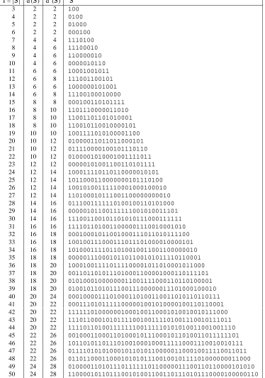
The curve on Fig. 1 (and its magnified version, Fig. 2) shows, for eachl ∈[3::405], the autodistance and the reverse autodistance of the best double synchronizing sequence found for the lengthlby simulated annealing. The autodistance can be compared to up (l), also shown on the figures. Table 1 reproduces part of these results.
5.2.1 The autodistance
For 3l42, the autodistance of the examples is, with the exceptions ofl= 27 andl= 39, equal to up (l). For the particular cases ofl= 27 andl= 39, exhaustive searches showed that there are no synchronizing sequences with autodistance equal to up (l)
1; the examples found
for these two values oflare therefore optimal.
We are thus certain that, forl 42 (as well as for l = 45, 46, 49, 50, 54, see Fig. 2), the simulated annealing program actually found optimal synchronizing sequences. For these values, with the exceptions of l = 27 and l = 39, the upper bound of Theorem 1 is exact. For l= 27 andl = 39, the maximal autodistance is less than up (l), and Theorem 1 could be improved to take this fact into account.
According to Theorem 5, for lengths of the forml= 2 n
1, some sequences achieve the upper bound up (l). Therefore, forl = 63;127;255, the simulated annealing program found
1
Forl = 39, the exhaustive search was performed by Mark Shand [8] using a carefully optimized search
50 100 150 200 250 300 350 400 50
[image:18.708.174.555.161.386.2]100 150 200
Figure 1: Autodistance and reverse autodistance of example sequences as a function of their lengthsl. The lower line shows the autodistance of the best double synchronizing sequence found by simulated annealing for each length. The upper, dotted line shows the reverse autodistance of the same sequences. The middle, perfectly regular line shows up (l).
10 20 30 40 50
10 20 30
[image:18.708.180.555.485.723.2]l=jSj d (S) d 0
(S) S
3 2 2 100
4 2 2 0100
5 2 2 01000
6 2 2 000100
7 4 4 1110100
8 4 6 11100010
9 4 6 110000010
10 4 6 0000010110
11 6 6 10001001011
12 6 8 111001100101
13 6 6 1000000101001
14 6 8 11100100010000
15 8 8 000100110101111
16 8 10 1101110000011010
17 8 10 11001101101010001
18 8 10 110010110010000101
19 10 10 1001111010100001100
20 10 12 01000011011011000101
21 10 12 011110000100101110110
22 10 12 0100001010001001111011
23 12 12 00000101001100110101111
24 12 14 100011110110110000010101
25 12 14 1011000110000000101110100
26 12 14 10010100111110001000100010
27 12 14 110100010111001100000000010
28 14 16 0111001111110100100110101000
29 14 16 00000101100111111001010011101
30 14 16 111001100101101010111000111111
31 16 16 1111011010011000001110010001010
32 16 18 00010001011001000111011010111100
33 16 18 100100111000111011101000010000101
34 16 18 1010001111011010010011001100000010
35 18 18 00000111000101101100101011110110001
36 18 20 100010011110111100001011010001011000
37 18 20 0011011010111010001100001000110111101
38 18 20 01010001000000011001111000110110100001
39 18 20 010010110101110011100000011101000100010
40 20 24 0001000011101000110100110011010110110111
41 20 22 00011101011111000001001010000100110110001
42 20 22 111111010000001000100110001010010010111000
43 20 22 1110110001010111100100111101001110010111011
44 20 22 11110110100111111100111110101010011001001110
45 22 26 001000110001101000101110001011010011011111101
46 22 26 1011010110111010010001000111110001110010010111
47 22 26 01111010101000101101011000001100010011110011011
48 22 26 011011000110001010101110010010111101000000011000
49 24 28 0100001101011101111110110000011100110110000101010
[image:19.708.176.550.190.723.2]50 24 28 11000010110111001010011001101110101110000100000110
only sub-optimal synchronizing sequences.
Forl= 43;44;48, by systematically searching through a significant fraction off0;1g l
, Mark Shand [8] found words achieving up (l); the best examples found by simulated annealing for these values oflare therefore non-optimal.
For all values of l not mentionned above, we do not know whether the synchronizing sequences found using simulated annealing are optimal; we do not know, either, whether up (l) is the exact upper bound for those values. Unlike forl 44, the exhaustive search, which costsO(2
l
) in time, cannot be applied to answer these questions.
5.2.2 The reverse autodistance of optimal synchronizing sequences
Lemma 3 and Theorem 3 imply that the examples found forl∈f3::15, 17::21, 23, 24, 26, 28::33, 35, 37, 42gare double-optimal synchronizing sequences.
As indicated in Section 5.2.1 above, for l = 27 there are no words S ∈ f0;1g l
with d (S) = up (l); a computation analogous to the these in the proof of Theorem 3 shows that there is also no word of this length with d (S) = d
0
(S) = up (l) 2. Therefore, the corresponding example is a double-optimal synchronizing sequence.
Forl= 16;22;25, exhaustive searches showed that there is no wordS ∈f0;1g l
satisfying d (S) = d
0
(S) = up (l); the corresponding examples are therefore double-optimal synchronizing sequences.
For l ∈ f34, 36, 38, 40, 41, 45, 46, 49, 50, 54g, the examples found are optimal synchronizing sequences, but the author has not been able to establish whether they are double-optimal.
6 Double Synchronizing Sequences of Lengthl!+∞
6.1 The result
Theorem 6 (double synchronizing sequences for largel) Let ∈ R; 0 < < 1. There exists a function": N2+!R+such that lim+∞"= 0 and that for everyl∈N,l 3, there are at least2
l
distinct wordsS∈f0;1g l
satisfying
up (l) l "(l)d (S)d 0
(S)up (l) +l "(l)
6.2 How the proof is organized
The proof of Theorem 6 is long. Let us summarize it here.
Section 6.5 contains auxiliary lemmas, which recall generally known mathematical facts. Sections 6.6–6.9 contain the proof of the first capital lemma.
In Section 6.6, we choose a function"which, as we will prove, satisfies both capital lemmas (and thus the theorem). We define then the setE f0;1g
l
of words whose autodistance is less than up (l) "(l)l, and we represent it as equal to the union of a family of sets calledE
p;D. Then, in Sections 6.7 and 6.8, we establish intermediate results which will enable us to estimate the cardinals of the setsE
p;D. Finally, in Section 6.9, we use these results to prove thatjEj
1
2 2
l
, from what the first capital lemma results.
In Section 6.10, rather than fully describing the proof of the second capital lemma, we simply indicate in which ways it differs from the proof of the first capital lemma.
6.3 The two capital lemmas
Theorem 6 follows in a straightforward way from the two following lemmas.
Capital Lemma 1 (autodistance for highl) Let∈R; 0<<1. There exists a function " : N2+ ! R+ such that lim+∞" = 0 and for every l ∈ N, l 3, there are at most
1
2 2
l distinct wordsS∈f0;1g
l
such that
d (S)<up (l) l "(l)
Capital Lemma 2 (reverse autodistance for highl) Let∈R; 0< <1. There exists a function ": N2+ ! R+ such that lim+∞" = 0 and for everyl ∈ N,l 3, there are at most
1
2 2
l
distinct wordsS∈f0;1g l
such that
up (l) +l "(l)<d 0
(S)
6.4 Conventions
We make, for the whole proof, the following assumptions about the numbersl,p,a,band and about the setsDandP:
l∈N2+; 3l p∈Z; 1pl =2
a∈N; 1a
b∈N; 2b
∈R; 0<<1=2 D[0::l)
These assumptions are valid in lemmas and auxiliary definitions which are part of the proof. They will not be recalled there. For instance, the following
Example Lemma 1 For every∈R such that 0<<1=2 and for everyn∈Z, ≠ n.
will be abbreviated to
Example Lemma 2 For everyn∈Z, ≠ n.
6.5 Auxiliary lemmas
Lemma 4 (approximation of
n d
) For everyn;d∈N,
d 1=2
n 1 implies n d 2 n e 3 n
Proof outline: Let us define q = b(1=2 =2)nc. Using the well-known equality n r = n!
r!(n r)!
, we can then state the following:
∀(r∈[d::q)) n r 1 1 + n r+ 1
n d 1 1 + n=2 n q n d 1 1 + n=2 2n n d e 3 n 2n 2
Auxiliary Definition 8 (familiesF i) For
i ∈ [0::lup) and x ∈ h
0:: l lup
, we define the numbers
F ix= (
xp+i) modl which form the families
F i= (
F ix)0
x< l lup The numbers F
ixand the families F
i depend on the numbers
landpbut, for simplicity,l andpdo not appear as indices in their notation.
Lemma 5 (fundamental property ofF
i) For every
i ∈ [0::lup), the family F
i contains exactly once every element of the setA
i = ((
Proof outline: We call Im(F
i) the image of the family F
i, namely Im(F
i) = n F ix 0 x< l lup o
For everyx;y∈ h
0:: l lup
, the equationF ix=
F
iy is equivalent to ∃(k∈Z); (x y)
p lup
=k l lup which, thanks to the Gauss theorem [6], impliesx y ∈
l lup
Z. Since l lup
<x y < l lup
, we getx=y. All the elements of the familyF
iare therefore distinct and the family contains every element ofA
iat most once. Since all the elements of F
i are distinct, the set Im( F
i) contains l lup
elements; A i and Im(F
i) have therefore the same number of elements. Since, as the reader may easily verify, Im(F
i)
A
i, we get Im( F
i) = A
i. The family F
i contains then each element of A
i at least once and contains no elements from outsideA
i.
2
Lemma 6 (parity of the cardinal) IfAandB are finite sets,jA4Bjhas the same parity as
jAj+jBj. In other words,
jA4Bj≡jAj+jBj (mod 2)
The proof is left to the reader.
6.6 The setsE p;D
Letbe defined as in Capital Lemma 1. We define then
0
(l) = 1 lnl
+2 l
lnlln 2l
2
1
!
1=3
" 0
(l) = 0
(l) + 2 lnl
l +1
l
"(l) = (
" 0
(l) if " 0
(l)<1=2 and 0
(l)<1=2 1 otherwise
The functions 0
," 0
and"are then strictly positive, and satisfy
lim+∞ 0
= 0 lim+∞"
0 = 0 lim+∞" = 0
(the easy, computational proofs of these facts are not reproduced here)
To prove Capital Lemma 1, it is now sufficient to establish, for everyl, the property that there are at most 1
2 2
l
distinct wordsS ∈f0;1g l
Forlsuch that" 0
(l)1=2 or 0
(l)1=2, we have"(l) = 1 and the property trivially holds. We suppose therefore, for the rest of the proof, that"
0
(l)<1=2 and that 0
(l) <1=2, and we establish the property in this case.
Define
= up (l) l "(l) (19)
E =
n
S ∈f0;1g l
d (S)< o
(20) The property to be proven can then be expressed by the relation
jEj
1
2 2 l
(21) By Definition 1, equation (20) can be rewritten as
E= n
S ∈f0;1g l
∃(q ∈[1::l)) d S; q( S) < o (22) From the definition of the Hamming distance, it is easy to show that for everyq∈Z and every S ∈f0;1g
l , d S; q( S)
= d S; l q(
S)
and (22) is equivalent to
E = n
S ∈f0;1g l
∃ p∈
1::bl =2c d S; p( S) < o (23) We then define
E p =
n
S ∈f0;1g l d S; p( S) < o (24) Relation (23) can then be rewritten
E= bl=2c
[
p=1 E
p (25)
Let us define, forS ∈f0;1g l
, the set of differencesD S;p: D
S;p = n
i∈[0::l) S[i] ≠ p(
S)[i] o
(26)
D S;p =
n
i∈[0::l) S[i] ≠ S[(i+p) modl] o
(27) and, for anyD, let
E p;D=
n
S ∈f0;1g l D S;p= D o (28) Then (24) may be rewritten as
E p = [ jD j< E p;D (29)
From equations (25) and (29), we can deduce
jEj bl=2c
X p=1 X jD j< jE p;D j (30)
The rest of this proof consists in bounding the number of terms in this sum and in estimating jE
p;D
6.7 More auxiliary lemmas
Auxiliary Definition 9 (functions'[i] and expressionf(D ;i;j)) For i ∈ N, let us define the functions';'[i] :f0;1g!f0;1g
'(x) = 1 x '[0] (x) = x
'[i+ 1] (x) = '[i]'(x) Fori∈[0::lup) andj∈
h 0::
l lup
i
, we define
f(D ;i;j) = (F
ix)0 x<j
D
The expression f(D ;i;j) depends on l andp, which, for simplicity, do not appear there as indices.
Lemma 7 (relation betweenS[i],S[j] andD
S;p) Let
S ∈ E
p;D. Then, for 0
i <lup and 0j
l lup
, we have
S[(i+pj) modl] ='[f(D ;i;j)] (S[i])
Proof: First, observe that forneven,'[n] (x) =xand fornodd,'[n] (x) = 1 x.
We will prove the lemma by induction onj; the verification that the lemma holds forj= 0 is left to the reader.
Let us assume the lemma true forj(with 0 j < l lup
) and prove it forj+ 1. Under the lemma’s hypotheses, the fact thatS ∈E
p;D(which implies D=D
S;p) and relation (27) let us state:
if (i+pj) modl∈D, S[(i+p(j+ 1)) modl] = 1 S[(i+pj) modl] otherwise, S[(i+p(j+ 1)) modl] =S[(i+pj) modl]
which may be expressed as follows
S[(i+p(j+ 1)) modl] = '
jD\f(i+pj) modl gj
(S[(i+pj) modl]) = '[f(D ;i;j+ 1) f(D ;i;j)] (S[(i+pj) modl]) = '[f(D ;i;j+ 1) f(D ;i;j)] ('[f(D ;i;j)] (S[i]))
S[(i+p(j+ 1)) modl] = '[f(D ;i;j+ 1)] (S[i])
2
Lemma 8 (someE
p;Dare empty) If, for some
i∈[0::lup), the numberj((lup)Z +i)\D j is odd, thenE
Proof: Leti∈[0::lup) and letj((lup)Z +i)\D)jbe odd. By Lemma 5, we get
jF i
j D
= j(((lup)Z +i)\[0::l)) \ D j = j((lup)Z +i)\D j
jF i
j D
is then odd. Applying Lemma 7, for everyS∈E
p;Dwe get then
S[i] = S
i+p l lup
modl
S[i] = '
f(D ;i; l lup
)
(S[i])
S[i] = '
jF i
j D
(S[i])
S[i] = 1 S[i] (sincejF i
j D
is odd)
which is impossible. Therefore,S∈E
p;Dis true for no
SandE
p;D=∅.
2
Lemma 9 (E
p;Dhas at most 2 lup
members) For everyS 0∈
f0;1g lup
, there exists at most oneSsuch thatS∈E
p;Dand the leftmost factor of
Sof lengthlupis equal toS 0
.
Proof: LetS ∈E p;Dand
k∈[0::l). Letibe the remainder in the division ofkbylup. Since 0i<lupandk ∈((lup)Z +i)\[0::l), Lemma 5 implies that for somej∈
h 0::
l lup
, we havek= (i+pj) modl. We can then apply Lemma 7 to get:
S[k] ='[f(D ;i;j)] (S[i])
This formula shows that every bit inS can be determined as a function ofl,p,Dand one of thelupleftmost bits ofS. Therefore, for any given values ofl,pandD, the left factor ofS
of lengthlupuniquely determinesS. 2
6.8 The setsD d;p
For anyd∈N, let us define
D d;p =
n
D jD j<d∧E
p;D ≠ ∅ o
(31)
(the setD
d;pdepends on
l, but for simplicitylwill not appear as an index in its notation) We can rewrite equation (30) as follows:
jEj bl=2c
X
p=1 X
D∈D ;p
jE p;D
By Lemma 9, for everyD∈D ;p,
jE p;D
j2 lup
and equation (32) implies
jEj bl=2c
X p=1 jD ;p j2 lup (33)
Let us find two different (and both useful) upper bounds onjD ;p
j. SinceD
;pis only composed of subsets of [0
::l) containing less thanelements, we get
jD ;p j X 0x< l x (34)
and we can easily verify that the hypotheses of Lemma 4 hold (for= 0
(l)); in this way we get the first upper bound onD
;p
jD ;p
jl e
0
(l)
3
l 2l
(35)
Let us compute the second upper bound onD
;p. To simplify notation, we define the two intervalsI andJ:
I = [0::a(b 1)) J = [a(b 1)::ab) Auxiliary Definition 10 (setsD
0 d;a;b;P
) For everyd∈N, let
D 0 d;a;b;P denote the set of sets D
0
[0::ab) such that jD 0
j < d and, for every i ∈ [0::a), jD
0
\(aZ +i)j+jP \(aZ +i)jis even.
Lemma 10 For everyd∈N,
D 0 d;a;b;P 2
a(b 1)
(36)
Proof: Since the setIhasa(b 1) elements, there are at most 2 a(b 1)
possible sets of the form D
0
\I. To prove the lemma, it will therefore suffice to establish that for fixedd,a,bandP, and under the condition thatD
0∈ D
0
d;a;b;P, the set D
0
\Iuniquely determinesD 0
. For everyi,D
0
\(aZ +i) is the disjoint union ofD 0
\I \(aZ +i) andD 0
\J\(aZ +i), therefore
D 0
\(aZ +i) = D 0
\I\(aZ +i) + D 0
\J\(aZ +i) The number D 0
\I \(aZ +i) + D 0
\J\(aZ +i) +
jP \(aZ +i)j is therefore even. The parity ofjD
0
\J\(aZ +i)jis hence determined byD 0
On the other hand, we have
J \(aZ +i) =fi+a(b 1)g Therefore,
D 0
\J\(aZ +i)
even implies D
0
\J\(aZ +i) =∅
D
0
\J\(aZ +i)
odd implies D
0
\J\(aZ +i) =fi+a(b 1)g In this way,D
0
\I uniquely determinesD 0
\J\(aZ +i) for everyi. The (easy to verify) equality
D 0
= (D 0
\I)[ a 1
[
i=0 D
0
\J\(aZ +i)
implies then thatD 0
\Iuniquely determinesD 0
. 2
Lemma 11 For everydsuch that 0d(1=2 )ab b,
D
0 d;a;b;P
ae
3
a
2ab+b a
(37)
Proof: For every value ofa, we will prove the lemma by induction onb.
First, we need to verify the lemma for b = 2. This verification, when fully described, is extremely long. For this reason, we will omit here numerous computational details.
For any fixedd,aandP satisfying lemma’s hypotheses and forb= 2, we considerD 0
as a variable satisfyingD
0∈ D
0
d;a;2;P and we estimate the number of values that D
0
can take (this number is obviously equal to
D
0 d;a;2;P
). We define the setsU andV:
U =
n
i∈I jP \(aZ +i)j∈2Z o
V =
n
i∈I jP \(aZ +i)j∉2Z o
It is easy to see that ifjVj>d, thenD 0 d;a;2;P
=∅and the lemma holds. We suppose therefore thatjVjdand verify the lemma in this case only.
Let us quote the following, easy to establish, relations:
U [V = [0::a)
U \V = ∅
jUj+jVj = a
U +a J
Leti∈V. The cardinal ofD 0
\(aZ +i) is then odd and, sinceD 0
\(aZ +i)fi;a+ig, we get
a+i∈D 0
() i∉D
0
i∈D 0
a () i∉D
0
(38)
From here, we can deduce that
V \(D 0
a) = V D
0 (V +a)\D
0
= (V D 0
) +a (39)
Therefore,V \D 0
uniquely determines (V +a)\D 0
. By remarking thatV \D 0
can take at most 2jVj
different values, we conclude that (V [(V +a))\D 0
can only take 2jVj
different values.
From relation (39) we get
(V +a)\D 0 +
V \D 0
=jVj
V and V +a being disjoint, we conclude that j(V [(V +a))\D 0
j = jVj. Since the sets V [(V +a) andU [(U+a) are disjoint, we finally get
(U [(U +a))\D 0 +
(V [(V +a))\D 0 < d (
U [(U+a))\D 0
< d jVj (40)
A relation concerningU and analogous to (39) can be established:
(U+a)\D 0
= (U \D 0
) +a (41)
and can be used to conclude thatU \D 0
uniquely determines (U +a)\D 0
.
Relation (41), together with the fact thatU andU +aare disjoint, leads to the conclusion that
U \D 0 =
(U+a)\D 0 = 1 2
(U [(U+a))\D 0
U \D 0
<
d jVj
2 (by (40))
Since U\D 0
is a set containing less than (d jVj)=2 elements chosen among thea jVj elements ofU, it can take at most
X
0k <(d jVj)=2
a jVj k
different values; the same is true concerning (U [(U+a))\D 0
(since this set is determined in a unique way byU\D
From the fact that
D 0
= (U [(U+a))\D 0
[ (V [(V +a))\D 0
we finally deduce thatD 0
can take no more than
X
0k <(d jVj)=2
a jVj k
2jVj
different values; then
D
0 d;a;2;P
a
a jVj b(d jVj)=2c
2jVj
(42)
We can verify the following relations (remember thatjVjd)
0
d jVj
2
1
2
a a jVj
(a jVj) 1
0 < a a jVj
< 1 2
which, together with (42), enable us to use Lemma 4 and obtain
D
0 d;a;2;P
ae
3 a
3 (a jVj)3
(a jVj) 2a jVj
2jVj
from that we deduce that (37) holds and we thus end the verification forb= 2. Now, we suppose thatb3 and that the lemma holds forb
0
= b 1. Supposing thata,d, andP satisfy the lemma’s hypotheses, let us establish relation (37). LetD
0∈ D
0 d;a;b;P
. We can splitD
0
into the union of two disjoint subsetsD1andQ:
D1 = D
0 \I
Q = D
0 \J By definition ofD
0 d;a;b;P
, for everyi∈[0::a) we have
D 0
\(aZ +i)
+jP \(aZ +i)j∈2N
this can be rewritten as
jD1\(aZ +i)j+jQ\(aZ +i)j+jP \(aZ +i)j∈2N and, by Lemma 6,
jD1\(aZ +i)j+j(P4Q)\(aZ +i)j∈2N (43) The facts thatD1Iand thatjD1j+jQj=jD
0
j, together with relation (43), enable us to state
D1∈D 0
We have therefore established that everyD 0∈
D 0 d;a;b;P
is the union of someQJand some D1∈D
0
d j Qj;a;b 1;P4Q . Then, D 0 d;a;b;P [ QJ n
D1[Q D1∈D 0
d jQj;a;b 1;P4Q o D 0 d;a;b;P X QJ D 0
d j Qj;a;b 1;P4Q
(44)
Let us split the sum (44) into two termsXandY: D 0 d;a;b;P
X+Y
X =
X
QJ jQj<(1=2 )a 1
D
0
d j Qj;a;b 1;P4Q Y = X QJ jQj(1=2 )a 1
D
0
d j Qj;a;b 1;P4Q
The sumX is indexed by subsets ofJ having less than (1=2 )a 1 elements. Lemma 4 implies then that the number of terms in the sum is less than or equal to
X
0i<(1=2 )a 1 a i ae 3 a 2a
From Lemma 10, we deduce that each term inXis less than or equal to 2 ab 2a
; therefore,
Xae
3
a 2ab a
(45) The sumY, being indexed by subsets ofJ, contains at most 2
a
terms. Each term is of the form
D
0
d jQj;a;b 1;P4Q where
d jQj(1=2 )a(b 1) (b 1)
After straightforward verifications, the induction hypothesis (Lemma 11 applied for b 1) may be applied to give
D
0
d jQj;a;b 1;P4Q ae 3 a
2a(b 1)+(b 1) a
Therefore,
Y ae
3
a
2ab+(b 1) a
(46) and D 0 d;a;b;P ae 3 a 2ab a
+ae
3
a
2ab+(b 1) a D 0 d;a;b;P ae 3 a
2 The definition ofD
;p, together with Lemma 8, imply that D ;p D 0 ;lup; l lup ;∅
; if we set
=
0
(l), Lemma 11 implies
jD ;p
jle
0
(l)
3(
lup) 2l+
l lup
lup
(47) which is our second upper bound onD
;p. 6.9 Conclusion
Let us use the two bounds (35) and (47) to estimate the sum described in (33). For lup
l
lnl
, we have (by (35))
jD ;p j2 lup le 0
(l)
3
l 2l+lup
jD ;p j2 lup le 0
(l)
3
l 2l+
l
lnl (48)
Forlup> l
lnl
, we use (47), which implies,
jD ;p j2 lup le 0
(l)
3(
lup) 2l+
l lup jD ;p j2 lup l 2 e 0
(l)
3 l
lnl2 l
(49) For every term in the sum (33), either (48) or (49) holds. Therefore,
jEj
bl=2c X p=1 max le 0
(l)
3
l 2l+
l lnl ; l 2 e 0
(l)
3 l
lnl2 l
jEj max
l 2 e 0
(l)
3
l 2l+
l lnl ; l 3 e 0
(l)
3 l
lnl2 l
(50)
From (50), using the definition of 0
, we get (after a tedious computation) relation (21). 2
6.10 The proof of Capital Lemma 2
Let us describe the modifications that the proof of Capital Lemma 1 (Sections 6.6–6.9) should undergo in order to become a proof of Capital Lemma 2. Note that the function"used in both proofs is the same.
By analogy with the objectsandE(see (19) and (20)), we define
= up (l) +l "(l)
E =
n
S∈f0;1g l
d0
(S)> o
(51)
The property to be proven (corresponding with (21)) can then be expressed by the relation (analogous to (21))
By analogy with (34), we get E
bl=2c X p=1 X jD j> jE p;D j (53)
By analogy withD
d;p(see (31)), we define for any d∈N,
D d;p =
n
D jD j>l d∧E
p;D ≠ ∅ o
(54)
Then, in the same way as relation (34) is obtained, we get D ;p X
l <xl l x X 0x< l x
which, in turn, leads us to the first upper bound onD
;p(analogous to (35)): D ;p l e 0
(l)
3
l 2l
(55)
In order to obtain the second upper bound onD
;p(analogous to (47)), we use Lemma 8 and get, for alli∈[0::lup),
D∈D ;p =
) j((lup)Z +i)\D j∈2Z D∈D
;p =
) j((lup)Z +i)\([0::l) D)j+j((lup)Z +i)\[0::l)j∈2Z (56) The definition ofD
;p(formula (54)) implies that D∈D
;p=
)j[0::l) D j (57)
From (56) and (57), and from Auxiliary Definition 10, we get
D ;p
n
D[0::l) [0::l) D ∈ D 0 ;lup;
l lup
;[0::l) o
Finally, by observing that the function transforming D (forD [0::l)) into [0::l) Dis bijective, we obtain
D ;p D 0 ;lup; l lup
;[0::l) and using Lemma 11, we get the second upper bound onD
;p(analogous to (47)): D ;p le 0
(l)
3(
lup) 2l+
l lup
lup
(58)
The two bounds (55) and (58) enable us to derive (52) in the same way as (21) is obtained in
References
1. Patrice Bernard. Corpac 900, une autre approche. Technical Report 06 10 00 MGT 003, TECSI, 29, rue des Pyramides, 75001 Paris (May 1981).
2. Richard E. Blahut. Digital Transmission of Information. Addison-Wesley (1990).
3. S. Kirkpatrick, C. D. Gelatt, Jr., and M. P. Vecchi. Optimization by simulated annealing. Science, 220:671–680 (1983).
4. Rudolf Lidl and Harald Niederreiter. Introduction to Finite Fields and their Applications. Cambridge University Press, Cambridge, UK (1986).
5. Raymond L. Pickholtz, Donald L. Schilling, and Laurence B. Milstein. Theory of spread-spectrum communications — a tutorial. IEEE Transactions on Communications, COM-30(5):855–884 (May 1982).
6. E. Ramis, C. Deschamps, and J. Odoux. Cours de Math´ematiques Sp´eciales, volume 1, section 3.3.2, paragraph 3e. Masson, Paris (1979).
7. Dilip V. Sarwate and Michael B. Pursley. Crosscorrelation properties of pseudorandom and related sequences. Proceedings of the IEEE, 68(5):593–619 (May 1980).
The following documents may be ordered by regular mail from:
Librarian – Research Reports Digital Equipment Corporation Paris Research Laboratory 85, avenue Victor Hugo 92563 Rueil-Malmaison Cedex France.
It is also possible to obtain them by electronic mail. For more information, send a message whose subject line [email protected], from within Digital, todecprl::doc-server.
Research Report 1:Incremental Computation of Planar Maps. Michel Gangnet, Jean-Claude Herv ´e, Thierry Pudet, and Jean-Manuel Van Thong. May 1989.
Research Report 2:BigNum: A Portable and Efficient Package for Arbitrary-Precision Arith-metic. Bernard Serpette, Jean Vuillemin, and Jean-Claude Herv´e. May 1989.
Research Report 3: Introduction to Programmable Active Memories. Patrice Bertin, Didier Roncin, and Jean Vuillemin. June 1989.
Research Report 4: Compiling Pattern Matching by Term Decomposition. Laurence Puel and Asc ´ander Su ´arez. January 1990.
Research Report 5:The WAM: A (Real) Tutorial. Hassan A¨ıt-Kaci. January 1990.
Research Report 6:Binary Periodic Synchronizing Sequences. Marcin Skubiszewski. May 1991.
Research Report 7: The Siphon: Managing Distant Replicated Repositories. Francis J. Prusker and Edward P. Wobber. May 1991.
Research Report 8: Constructive Logics. Part I: A Tutorial on Proof Systems and Typed
-Calculi. Jean Gallier. May 1991.
Research Report 9:Constructive Logics. Part II: Linear Logic and Proof Nets. Jean Gallier. May 1991.
Research Report 10:Pattern Matching in Order-Sorted Languages. Delia Kesner. May 1991.
Research Report 13:Functions as Passive Constraints in LIFE. Hassan A¨ıt-Kaci and Andreas Podelski. May 1991.