Virtual Machine and Code Generator for PLC Systems

(1)

Virtual Machine and Code Generator for

PLC-Systems

A Thesis submitted to the University of East London for the degree of Master of Philosophy

Thomas Gasser Dipl. El Ing. FH

Student Number: 0537311

Supervisor

Dr. D. Xiao, University of East London

(2)

Acknowledgments

This thesis is the result of six interesting years of research in the domain of PLC-Systems in the area of building automation, building control.

Many thanks are going to Prof. Dominic Palmer-Brown for his assistance and encouragement in the early stages of my work.

I wish to express my gratitude to my Director of Studies Dr. David Xiao for his continuous and effective guidance, and his valuable comments. He was a source of very helpful, constructive criticism.

Special thanks go to Prof. Dr. Harald Wild, who encouraged and supported me in the past seven years. His guidance, his critique and his friendship are most valuable to me!

(3)

Abstract:

In the programming of PLC-Systems (PLC = Programmable Logic Controller) in building automation there were no vital changes over the past few years. Most users of PLC-Systems in building automation do the programming in FBD (functional block diagram). The users always start their projects with the programming of the PLC software. After that the HMI (Human Machine Interface) or the SCADA-System (Supervisory Control And Data Acquisition) are added as subsequent Tasks. Programming tools like CoDeSys build on this bottom up approach. Most of the time the user has to cope with different tools for the different tasks and the programming tools are built for a specific hardware. Almost every PLC manufacturer has its own implementation of the IEC 61131 standard with various interpretations. So a change of hardware means that the programming tool, the way how to program the PLC-System, the HMI tool and the SCADA tool changes. The interfaces between the tools are sometimes pretty clumsy and software, generated with these tools, is often not easily transferred to the PLC-System of another PLC-System manufacturer.

This investigation proposes a top down approach to a project. For the first time the starting point of a project will be the plant diagram. The programming will be intuitively done in the plant diagram. Template objects (e.g. for pumps) created with the object orientated paradigm will be used to accomplish this task. The created PLC software will run in a virtual machine on the PLC-System and thus will be reusable on PLC-Systems of different manufacturers, which will eliminate the dependency on certain hardware.

(4)

(5)

Table of contents

ACKNOWLEDGMENTS ... 2

ABSTRACT: ... 3

TABLE OF CONTENTS ... 5

LIST OF FIGURES ... 11

LIST OF TABLES ... 13

LIST OF LISTINGS ... 14

CHAPTER 1: INTRODUCTION ... 16

1.1 Traditional approach: ... 17

1.2 New approach: ... 18

1.3 Objectives ... 19

CHAPTER 2: LITERATURE SURVEY ... 20

2.1 Code generation ... 20

2.1.1 Generative programming ... 21

2.2 Compiler construction ... 21

2.3 Virtual machines... 21

2.3.1 Process virtual machines ... 22

2.3.2 System virtual machines ... 22

2.4 PLC-Systems ... 22

2.4.1 Standardisation ... 23

2.4.2 Modeling ... 23

2.4.3 Special Articles ... 23

2.4.4 History ... 23

2.4.5 System design ... 24

2.4.6 Programming ... 26

2.5 SCADA-Systems ... 26

2.5.1 SCADA components ... 27

2.5.2 SCADA concepts ... 28

CHAPTER 3: RESEARCH METHODOLOGY ... 30

3.1 The Qt application framework ... 30

(6)

3.2.1 The server application (pTool) ... 30

3.2.2 The client application (sGen) ... 31

3.3 Inter-process communication ... 31

3.3.1 Systems used for Inter-process communication ... 31

3.3.2 Sockets ... 32

3.3.3 Named pipes ... 32

3.4 Data structures ... 32

3.4.1 Hashing ... 33

3.4.2 The hash function... 33

3.4.3 Hash table statistics ... 34

3.4.4 Collision resolution ... 34

3.4.5 Tree’s ... 39

CHAPTER 4: IMPLEMENTATION ... 40

4.1 Introduction ... 40

4.2 Initial position ... 40

4.2.1 Template object concept ... 40

4.2.2 Programming on the plant diagram ... 42

4.3 Current logical template objects ... 46

4.4 System design ... 47

4.4.1 System overview ... 48

4.4.2 Storage of the data... 48

4.5 Virtual machine on the PLC-System ... 48

4.5.1 Process virtual machine ... 49

4.5.2 Decode and dispatch Interpretation ... 49

4.5.3 Indirect threaded interpretation ... 50

4.5.4 Chosen type of virtual machine ... 50

4.5.5 Design of the virtual machine ... 51

4.5.6 Implementation of VM001 ... 52

4.6 The new logical template object ... 52

4.6.1 Design of the LTO01 ... 52

4.6.2 Implementation of LTO01 ... 55

4.7 Implemenation of the interpreter routines ... 55

(7)

4.7.3 Functionblock interface fbXor (skeleton only) ... 56

4.7.4 Real local variables (temporary data)... 56

4.7.5 Get the number of used inputs ... 57

4.7.6 Process the digital technology function ... 57

4.8 The Server Application pTool ... 61

4.8.1 pTool basics ... 61

4.8.2 Implementation overview ... 63

4.8.3 pTool commands... 67

4.8.4 The local server... 67

4.8.5 The configuration file pTool.ini ... 67

4.9 The Client Application, the code generator, sGen ... 68

4.9.1 sGen basics ... 68

4.9.2 The developed dll’s ... 69

4.9.3 The debug window ... 69

4.9.4 The sGen dialog ... 71

4.9.5 The VM generator ... 76

CHAPTER 5: TESTING ... 114

5.1 Testing environment ... 114

5.1.1 Details PLC-System ... 115

5.1.2 Details ProMoS NT ... 115

5.2 Testing tools ... 116

5.2.1 The online debugger ... 116

5.2.2 The watch window... 117

5.2.3 In code debugger ... 118

5.2.4 Debugging tools ... 119

5.2.5 Use of the new system in a real facility ... 120

5.2.6 Plant diagram before the use of the VM ... 121

5.2.7 Plant diagram using the VM ... 122

5.3 Testing procedure ... 123

5.4 Compiling test ... 123

5.5 Functional test ... 124

5.5.1 The plant overview diagram ... 124

5.6 Testing results ... 127

(8)

5.6.2 LTO001 OR-Gate ... 128

5.6.3 VM001 ... 128

5.6.4 Cycle time ... 128

CHAPTER 6: RESULTS AND DISCUSSION ... 130

CHAPTER 7: CONCLUSIONS ... 131

7.1 Achievement of objectives ... 131

7.1.1 Objective 1: To develop PLC software using the object orientated paradigm ... 131

7.1.2 Objective 2: To develop a generic SCADA-System FBD programming language ... 132

7.1.3 Objective 3: To develop a virtual machine for PLC-Systems ... 132

7.1.4 Objective 4: To develop a code generator for PLC-Systems which uses the definition files of a SCADA-System as input ... 132

CHAPTER 8: RECOMMENDATION AND FUTURE WORK ... 133

APPENDIX A SOURCE CODE VM001.SRC ... 138

APPENDIX B SOURCE CODE VMLIB.SRC ... 148

APPENDIX C SOURCE CODE LTO01.SRC ... 163

APPENDIX D SOURCES PTOOL ... 168

APPENDIX D I SOURCE CODE PTOOL.H ... 168

APPENDIX D II SOURCE CODE MAIN.CPP ... 170

APPENDIX D III SOURCE CODE PTOOL.CPP ... 171

APPENDIX D IV SOURCE CODE QCPROJECT.H ... 181

APPENDIX D V SOURCE CODE QCPROJECT.CPP ... 183

APPENDIX D VI SOURCE CODE QCPROJECTCOMMANDS.CPP ... 193

APPENDIX D VII SOURCE CODE STANDARDTREEMODEL.H ... 213

APPENDIX D VIII SOURCE CODE STANDARDTREEMODEL.CPP ... 214

APPENDIX E SOURCES PLIB ... 217

APPENDIX E I SOURCE CODE PLIB.H ... 217

(9)

APPENDIX E III SOURCE CODE PLIBRESSOURCES.CPP ... 230

APPENDIX E IV SOURCE CODE PLIBTOS.CPP ... 232

APPENDIX F SOURCES SGEN ... 242

APPENDIX F I SOURCE CODE SGEN.H ... 242

APPENDIX F II SOURCE CODE MAIN.CPP ... 246

APPENDIX F III SOURCE CODE SGEN.CPP ... 247

APPENDIX F IV SOURCE CODE DATAMACHINE.CPP ... 255

APPENDIX F V SOURCE QCDATATREE.H ... 273

APPENDIX F VI SOURCE CODE QCDATATREE.CPP ... 274

APPENDIX F VII SOURCE CODE RXPGENERATOR.CPP ... 278

APPENDIX F VIII SOURCE CODE VMGENERATOR.CPP ... 283

APPENDIX G SOURCES SGENLIB ... 303

APPENDIX G I SOURCE CODE SGENLIB.H ... 303

APPENDIX G II SOURCE CODE SGENLIB.CPP ... 305

APPENDIX H SOURCES PTSOCKETLIB... 318

APPENDIX H I SOURCE CODE PTSOCKETLIB.H ... 318

APPENDIX H II SOURCE CODE PTSOCKETLIB.CPP ... 319

APPENDIX H III SOURCE CODE PTCLIENTMACHINE.H ... 320

APPENDIX H IV SOURCE CODE PTCLIENTMACHINE.CPP ... 322

APPENDIX H V SOURCE CODE PTSERVERMACHINE.H ... 333

APPENDIX H VI SOURCE CODE PTSERVERMACHINE.CPP ... 335

APPENDIX H VII SOURCE CODE COMMON.H ... 348

APPENDIX I GENERATED IL-CODE ... 349

APPENDIX J CONFIGURATION FILES ... 354

APPENDIX J I PTOOL.INI ... 354

APPENDIX J II SGEN.INI ... 355

(10)

APPENDIX J IV SRCVMHEADER.INI ... 358

APPENDIX J V SRCVMFOOTER.INI ... 360

APPENDIX K VERSIONS PLC-SYSTEM ... 361

APPENDIX K I PLC-SYSTEM... 361

APPENDIX K II PROGRAMMING SOFTWARE PG5 ... 361

APPENDIX L VERSIONS PROMOS NT ... 367

(11)

List of figures

Figure 1.1-1: Traditional approach ... 17

Figure 1.2-1: New approach ... 18

Figure 2.4-1: PLC-System design ... 24

Figure 2.4-2: Data processing ... 25

Figure 2.5-1: Automation pyramid (http://www.al-pcs.com) ... 27

Figure 2.5-2: SCADA concept (www.promosnt.ch) ... 29

Figure 3.2-1: Software design ... 30

Figure 3.3-1: IPC over named pipe ... 32

Figure 3.4-1: Hash collision resolved by separate chaining (Wikipedia) ... 35

Figure 3.4-2: Hash collision by separate chaining with head records in the bucket array (Wikipedia) ... 36

Figure 3.4-3: Hash collision resolved by open addressing with linear probing (Wikipedia) ... 36

Figure 3.4-4: This graph compares the average number of cache misses required to look up elements in tables with chaining and linear probing (Wikipedia) ... 38

Figure 3.4-5: Qt model / view architecture ... 39

Figure 4.2-1: Logical plant diagram (runtime mode) ... 40

Figure 4.2-2: Logical plant diagram (programming mode) ... 42

Figure 4.2-3: Logical plant diagram (example connection) ... 42

Figure 4.2-4: Logical plant diagram (choose output signal) ... 43

Figure 4.2-5: Logical plant diagram (choose input signal) ... 43

Figure 4.2-6: Logical plant diagram (signals linked) ... 44

Figure 4.4-1: System overview... 48

Figure 4.5-1; Decode and dispatch interpretation ... 49

Figure 4.5-2: Indirect threaded Interpretation ... 50

Figure 4.5-3: Implemented virtual machine ... 50

Figure 4.6-1: Reduce cost of binary resources ... 54

Figure 4.8-1: System-Tray-Icon of the pTool application ... 61

Figure 4.8-2: Context menu of the pTool application ... 61

Figure 4.8-3: Project context menu ... 61

Figure 4.8-4: pTool: Project dialog ... 62

(12)

Figure 4.9-2: sGen: Debug window ... 70

Figure 4.9-3: sGen_Dialogue: Data-Tab ... 71

Figure 4.9-4: sGen: Program flow ... 72

Figure 4.9-5: sGen: Detail program flow for a command ... 73

Figure 4.9-6: sGen-Dialog: Tree tab ... 74

Figure 4.9-7: sGen-Dialog: Generator tab ... 75

Figure 4.9-8: VM generator state machine ... 76

Figure 4.9-9: Saia-Burgess VM code generator ... 82

Figure 4.9-10: Insert function block call for the VM001 TO ... 109

Figure 4.9-11: Insert new lines, VM footer and COB footer ... 110

Figure 4.9-12: Writting the generator template string to the file ... 111

Figure 4.9-13: The generated code for the VM ... 112

Figure 4.9-14: The qsmsCloseVmFile_entered() function ... 112

Figure 4.9-15: Final state of the generator machine is reached ... 113

Figure 5.1-1: The used test system ... 114

Figure 5.2-1: Saia online debugger ... 116

Figure 5.2-2: Saia watch window ... 117

Figure 5.2-3: Debugging tools ... 119

Figure 5.2-4: Plant diagram (Heating system) of the test plant ... 120

Figure 5.2-5: Plant diagram before the use of the VM ... 121

Figure 5.2-6: System overview in a real plant diagram ... 122

Figure 5.5-1: The plant overview diagram ... 124

Figure 5.5-2: Testing plant function 01 ... 125

Figure 5.5-3: Watch window 01 ... 126

Figure 5.5-4: Watch window 02 ... 126

Figure 5.5-5: Testing plant function 02 ... 127

(13)

List of tables

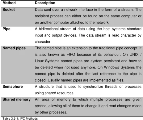
Table 3.3-1: IPC Methods ... 31

Table 3.4-1: Probing algorithms for open addressing ... 37

Table 4.2-1: Description of the TO ... 41

Table 4.2-2: Parts of a TO ... 41

Table 4.2-3: Colouring of the link lines ... 44

Table 4.3-1: Current LTO ... 46

Table 4.5-1: VM01: Parameters ... 51

Table 4.6-1: LTO01: Parameters ... 53

Table 4.7-1: Truth table for the XOR-Function ... 59

Table 4.8-1: pTool commands ... 67

Table 4.9-1: Developed DLLs ... 69

Table 4.9-2: Saia-Burgess configuration files ... 81

Table 5.1-1: Details PLC-System ... 115

Table 5.1-2: Details ProMoS NT ... 115

Table 5.2-1: Legend of the Plant diagram (Heating system) of the test plant . 120 Table 5.2-2: Legend of the Plant diagram before the use of the VM ... 121

Table 5.2-3: Legend of the System overview in a real plant diagram ... 122

Table 5.5-1: Legend of the The plant overview diagram ... 124

Table 5.5-2: Legend of the Testing plant function 01 ... 125

Table 5.6-1: Test results LTO001 ... 127

Table 5.6-2: Test results LTO001 ... 128

Table 5.6-3: Test results VM001 ... 128

(14)

List of listings

Listing 4.2-1: Generated Function Block call with parameters ... 46

Listing 4.6-1: Generated IL code for a binary conjunction ... 53

Listing 4.7-1: Functionblock interface fbAnd ... 55

Listing 4.7-2: Functionblock interface fbOr ... 56

Listing 4.7-3: Functionblock interface fbXor ... 56

Listing 4.7-4: Temporary data ... 56

Listing 4.7-5: Get input count ... 57

Listing 4.7-6: Prepare indexes ... 57

Listing 4.7-7: Check state of the input ... 58

Listing 4.7-8: Get logic information ... 58

Listing 4.7-9: Calculate the binary state used in the conjunction... 59

Listing 4.7-10: Processing of the digital technology function ... 59

Listing 4.7-11: Set the output of the LTO according to the conjunction result ... 60

Listing 4.8-1: load project (pseudocode) ... 63

Listing 4.8-2: execute command (pseudocode) ... 66

Listing 4.9-1: The main function of the sGen application ... 70

Listing 4.9-2: on_qpbGenerateVm_clicked() function ... 77

Listing 4.9-3: if_qsmsOpenVmFile_entered() function ... 79

Listing 4.9-4: The if_qsmsWriteHeader_entered() function ... 80

Listing 4.9-5: LTO generation: first run ... 83

Listing 4.9-6: LTO generation: second run ... 83

Listing 4.9-7: The createLtoHash() function ... 85

Listing 4.9-8: Helper registers ... 86

Listing 4.9-9: Generated code for the helper registers ... 86

Listing 4.9-10: Find DB address and assemble the allocation string ... 87

Listing 4.9-11: Generated code for the DB allocation ... 88

Listing 4.9-12: Retrieving of the number of DB elements ... 88

Listing 4.9-13: Getting the basic digital technology function configured for the LTO01 ... 89

Listing 4.9-14: Getting number of used inputs ... 90

Listing 4.9-15: Add the pointer to the input addresses to the DB ... 91

(15)

Listing 4.9-18: Final task of the LTO01 data retrieval ... 94

Listing 4.9-19: Write the generated code into the output string list... 94

Listing 4.9-20: Generated DB allocation code ... 95

Listing 4.9-21: Generate the FB calls ... 96

Listing 4.9-22: LTO01 Generator: Insert footer ... 97

Listing 4.9-23: Code generated by the LTO instance generator ... 98

Listing 4.9-24: VM generation: first run ... 99

Listing 4.9-25: VM generation: second run ... 100

Listing 4.9-26: The createVmHash() function ... 101

Listing 4.9-27: VM generation: third run step 1 ... 102

Listing 4.9-28: Generated VM header and helper registers ... 103

Listing 4.9-32: VM generation: third run step 4 (continued) ... 107

Listing 4.9-33: VM generation: ... 108

Listing 5.2-1: In code debugging ... 118

(16)

Chapter 1:

Introduction

In IEC 601131-3 Standard, IEC (2003), two graphical programming languages are defined, FBD and LD (Ladder diagram). Ladder logic is the oldest programming language for PLC-Systems. Programming in LD is done by copying the wiring diagram into the PLC-System programming tool. FBD consists of functional blocks which are connected together as it is done with logical gates.

Using the SCADA programming language, the logic operations are created a special programming mode in the background in while the process charts are drawn. The programming will adhere to the ISO 16484-3 Standard ISO (2005). Kandare et al (2003) shows an approach to PLC code generation based on a real world problem. An abstract functional block diagram is used to generate ST (Structured Text). ST is also part of the IEC 61131-3 Standard and is similar to high level languages as C++ or Java. With the SCADA programming language the conjunction data is saved in a definition file. The definition file is used by the code generator to create the source code for the selected PLC-System. Ways have to be found, to ensure that the generated PLC code is consistent and that in a PLC cycle every conjunction is evaluated in the correct order. The generator has to generate the correct PLC code for every possible solution a user may program, Aho et al (2007).

(17)

Virtual machines are covered in detail in Smith and Nair (2005). Performance was tested for the Saia-Burgess PLC-Systems.

Developing a programming language for SCADA-Systems which is independent of PLC hardware manufacturers is addressed. The SCADA-System programming language should be a kind of a functional block language as it is much easier for people to work with functional blocks and do the programming graphically than with an abstract programming language. LabVIEW from National Instruments or MATLAB from the MathWorks are good examples for graphical programming tools.

1.1

Traditional approach:

As shown in Figure 1.1-1: Traditional approach below the traditional approach in a building automation project stipulates, that first the software for the PLC is developed and as a subsequent task the visualisation is adapted to the PLC software.

(18)

1.2

New approach:

With the SCADA-System programming language a novel approach was chosen (Figure 1.2-1: New approach). The PLC software is developed using the object oriented paradigm. The whole engineering and the design of the plant diagrams is done with template objects. In special applications a huge amount of the PLC code which runs the plant can be generated. The necessary connections between the TO (Template Objects) is built afterwards in IL (Instruction list), FBD or ST. IL, FBD and ST are part of the IEC 61131-3 standard IEC (2003). In standard applications the whole PLC code can be generated without the need to create additional code to link the TO.

(19)

1.3

Objectives

There have been several objectives in this investigation.

1. To develop PLC software using the object oriented paradigm. 2. To develop a generic SCADA-System-FBD programming language 3. To develop a virtual machine for PLC-Systems.

(20)

Chapter 2:

Literature Survey

A literature survey has been conducted on the aims of this investigation. Several related fields of interest have been included into the survey to broaden the horizon of this investigation and to get new ideas for the programming of PLC controllers.

It was quite difficult to find any literature covering code generation for PLC controllers in the field of building automation. The object oriented paradigm and code generation in the area of building automation seems to be a rather unexplored field. Nevertheless there are some helpful sources.

2.1

Code generation

Some of the most helpful suggestions for this investigation were found in Code Generation in Action by Herrington (2003). Herrington (2003) describes the usefulness of code-generation and its pitfalls in detail. He explains code generation in a way that not only engineers understand it but also managers can see the usefulness of code generation and the possibility of saving time and money by the use of it. The savings stem from the saved time in the engineering process and the constant high quality of the generated software. Automatically generated software is much less susceptible to programming errors than software which is written and rewritten every time it is used by hand.

The spectrum of code generation reaches from very simple generators for the body of a C++ class and the appropriate header file to highly complex generators which automatically build database access software. Various generators can be assembled to highly sophisticated frameworks.

(21)

no longer of much relevance. This can of course bring forth new problems because of non-qualified or unexperienced programmers writing complex applications.

2.1.1 Generative programming

The concept of generative programming is described by Czarnecki and Eisenecker (2000). They show generative programming methods and Metaprogramming to be similar as the concepts mentioned in chapter 2.1 and introduced by Herrington (2003). Czarnecki and Eisenecker (2000) introduce Domain Engineering as a means to develop a workbench of reusable parts in a family of systems. Similar thoughts are expressed in “Software factories” by Greenfield and Short (2006). The authors of both works emphasize that generative methods are a powerful tool to improve the quality of software because of the use and reuse of well tested libraries and functions.

2.2

Compiler construction

A most enlightening source is the dragon book by Aho et al. (2007). He and his co-authors provide a very deep insight into the methods used in the field of compiler construction. Some of these methods are very helpful in this investigation. Chapter 3 of the dragon book covers lexical analysis which is, as Aho et al. (2007) states very clearly, the foundation of text processing of all sorts. Text processing is of great importance for this investigation.

Lexical analysis is the first phase in the compiling process. The lexical analyser is used to analyse the source code character by character. The source code is grouped into lexemes and a sequence of tokens for each lexeme is generated as output. This output is used as a basis for the parser which does the semantic analysis.

2.3

Virtual machines

Craig (2004) describes the formal background of virtual machines. As described by Smith and Nair (2005) there are two different kinds of virtual-machines.:

(22)

2.3.1 Process virtual machines

Smith and Nair (2005) states that a process virtual machine is used to provide a user application with a virtual application binary interface (ABI). Process virtual machines are used to emulate, replicate and optimize. In the past years the focus has been laid on high-level-language VM’s. The two best known examples for high-level-language process virtual machines are the Java VM architecture and the Microsoft common language infrastructure (CLI) which is used as the basis of the .NET framework. The main goal of this type of virtual machine is to achieve platform independence. This should enable cross platform portability of application software. To achieve this goal it is necessary to take into account, that the instruction set architecture (ISA) is different from one platform to another. Both of the above mentioned systems are using an ISA based on bytecode. For each target platform a virtual machine has to be developed to run the bytecode.

2.3.2 System virtual machines

These systems are the origin of the term virtual machine. These virtual machines are emulators for a whole system. A single host platform with its hardware is used by different VM’s whereupon every VM’s is given the illusion of having its own Hardware. A well-known type of system virtual machine is the hosted VM. In this type of VM the virtualization software runs on a host operating system like a standard, native application. The VM itself is controlled and executed by the virtualization software. All native drivers and system calls can be used by the VM through the virtualization software. The virtualization software brings an additional software layer into the system which may result in a degradation of performance. VMware is a well-known representative of such a system. Zhou and Chen (2009) shows an example of a system virtual machine for PLC-System, the main idea of the research is to simplify the process of to port an existing PLC-Software to another PLC-Hardware.

2.4

PLC-Systems

(23)

control a manipulator transportation control system. PLC-Systems are most flexible and can easily adapt to changing requirements.

2.4.1 Standardisation

PLC-Systems are subject to conditions of the IEC-61131 standard. As can be seen in IEC (2003) for most parts of a PLC-System strict guidelines are set by the standard but nevertheless there is some room for the manufacturers to distinguish themselves from their competitors.

2.4.2 Modeling

Basile et al. (2013) uses Petri nets as a means to model the system behaviour of complex industrial processes. Min et al. (2013) proposes a component based modelling system to tackle the problems of cyclic programs and to synthesize the necessary PLC code.

2.4.3 Special Articles

Today the protection systems of nuclear reactors are realized by the use of PLC-Systems. Yoo et al. (2013) proposes a platform change from PLC-Systems to FPGA (Field-Programmable Gate Array). Vogel-Heuser et al. (2013) compares the UML-based engineering versus the engineering by the use of IEC 61131-3 in teaching PLC-System programming.

2.4.4 History

(24)

2.4.5 System design

Figure 2.4-1: PLC-System design

(25)

Figure 2.4-2: Data processing

The data processing is normally split into three phases: • First phase: Read input data from the input modules.

• Second phase: Process the input data with the user program.

• Third phase: Write the changes of the output data to the output modules The first and the third phase are controlled by the operating system of the PLC-System. After reading the input values the operating system gives control to the user program which processes the newly acquired input data into the new output data. Then the operating system takes control and writes the updated output data to the output modules. After that a whole cycle has been run through and a new cycle starts with the first phase. There are systems with a fixed cycle time which are working with various tasks where every task can have its own, fixed cycle time. On the other hand there are systems where the cycle time is floating and therefore changing according to the user program.

(26)

input modules and writing to the output modules at the sametime. The cycle time is floating depending on the user program.

2.4.6 Programming

The different programming languages of a PLC-System are subject to Part 3 of the IEC61131 standard.

The standard describes five different PLC programming languages: • Sequential Function Chart (SFC)

• Instruction List (IL) • Structured Text (ST) • Ladder Diagram (LD)

• Function Block Diagram (FBD)

Every one of these programming languages is aimed at a different type of users. Historically the first and therefore oldest PLC programming language is the ladder diagram which provides means of copying the electrical wiring diagram into the PLC-System. It is therefore often used by technicians with a wide knowledge of hard-wired relay systems. Which programming language a programmer will select depends heavily on the field of his work, his skills of programming and his knowledge of the PLC-System used. In the field of building automation the programming language most frequently used is FBD because of its minimal training requirements. An attempt to create a system to verify the developed PLC programs was made by Biallas et al. (2012).

2.5

SCADA-Systems

SCADA is an acronym for Supervisory Control And Data Acquisition. As described in Wikipedia (2013) a SCADA-System is an industrial control system (ICS). As distinguished from other ICS, SCADA-Systems can be large scale and control multiple plants over large distances. SCADA-Systems are used in the infrastructure automation for instance in distributed heating systems.

(27)

[image:27.595.109.548.89.388.2]

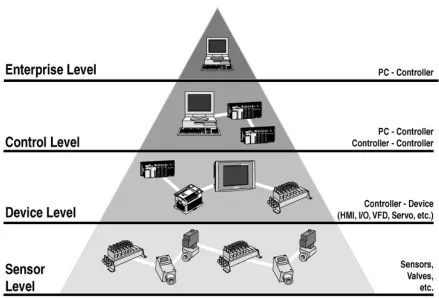
Figure 2.5-1: Automation pyramid (http://www.al-pcs.com)

2.5.1 SCADA components

As shown in Figure 2.5-1: Automation pyramid (http://www.al-pcs.com) there are various levels in an automation system. The automation pyramid is derived from the Open Systems Interconnection Model (OSI-Model).

Sensor, field level

Similarly as in the OSI-Model the lowest level, called layer in the OSI-Model, is where the interaction with the real-world takes place. This is the level where the actuators and sensors are placed.

Device level

(28)

SCADA-System. On this level simple Human Machine Interfaces (HMI) such as WEB-Panels or text based terminals can be found.

Control level

On this level the data exchange between the different controllers of a site or of various sites takes place. More sophisticated HMI-System can be found. They are part of the SCADA-System and therefore offer much more information to the operator of the site. On this level there are tools to thoroughly analyse the entities of a site and to optimise them to a very high level of efficiency.

Enterprise level

This level is optional and in smaller systems not present at all. Operators with their facilities distributed over a wide area use this level to realise centralised data acquisition in a control centre. This is usually done over the internet by the use of standard IT protocols and portal solutions. On this level automated data acquisition for accounting purposes takes place. Therefore the SCADA-Systems offer interfaces to accounting systems and business software.

2.5.2 SCADA concepts

(29)

[image:29.595.106.548.66.357.2]

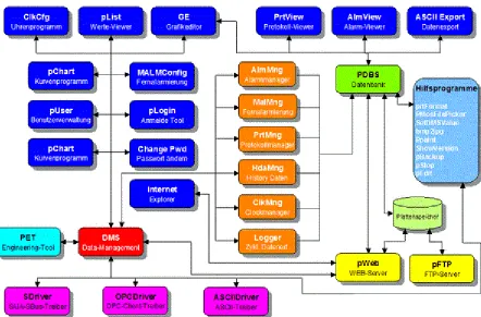
Figure 2.5-2: SCADA concept (www.promosnt.ch)

(30)

Chapter 3:

Research Methodology

3.1

The Qt application framework

For this investigation the application framework used is Qt. Qt is a cross-platform application and UI framework for developers using C++ or QML, a CSS & JavaScript like language. Qt’s Visual Studio 2010 plugin has been used to allow a smooth workflow between Qt and Visual Studio 2010.

3.2

The software design

The Software is designed as a Client / Server System. In this investigation the pTool-Application acts as the server in the System and the PLC code generator, sGen, is the client. Only the code generator for the Saia-Burgess PLC-Systems has been developed.

Figure 3.2-1: Software design

3.2.1 The server application (pTool)

(31)

3.2.2 The client application (sGen)

At the moment one client application has been developed. The application generates code for PLC-Systems from Saia-Burgess.

3.3

Inter-process communication

As described by Wikipedia (2013) Inter-process communication (IPC) is used in computing as a means for threads or processes to communicate among each other. IPC is a generic term for a class of methods to fulfil this task. The communicating processes can run on the same machine or can run on different machines connected by a network. In addition to the use as means of communication there is a second use of IPC which is the synchronization of processes or threads using shared resources.

3.3.1 Systems used for Inter-process communication

There are several different systems to implement IPC in an application.

Method Description

Socket Data sent over a network interface in the form of a stream. The recipient process can either be found on the same computer or on another computer attached to the network.

Pipe A bidirectional stream of data using the host systems standard input and output devices. The data stream is read character by character.

Named pipes The named pipe is an extension to the traditional pipe concept. It is also known as FIFO because of its behaviour. On UNIX / Linux Systems named pipes are system persistent and have to be deleted when not used anymore. On Windows Systems the named pipe is deleted after the last reference to the pipe is closed. Usually named pipes are implemented as files.

Semaphore A structure that is used to synchronize threads or processes using shared resources.

[image:31.595.91.554.376.763.2]

Shared memory An area of memory to which multiple processes are given access, allowing all of them to change it and read changes made by other processes.

(32)

3.3.2 Sockets

A socket is an endpoint in a line of communication, usually of an IPC. Gay (2000) describes sockets to be similar to the telephones used when calling someone else. The telephone represents the socket and the telephone network represents the network used by the sockets. In this investigation the easier to use named pipes were preferred to the use of sockets.

3.3.3 Named pipes

This investigation uses a QLocalSocket to implement IPC. On a Windows System the QLocalSocket is implemented as a named pipe. The implementation is done as a client-server system and therefore named pipes are working much like sockets.

Server (pTool)

Client (sGen)

Establish connection

Server (pTool)

command

Answer

Client (sGen)

Connection established

Figure 3.3-1: IPC over named pipe

3.4

Data structures

(33)

3.4.1 Hashing

For this investigation, the use of hashing in connection with hash tables is of interest. The use of hashing in cryptology has not been used in this work and therefore has not been researched.

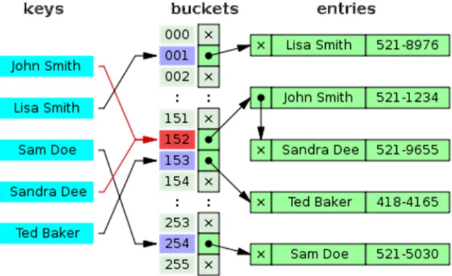
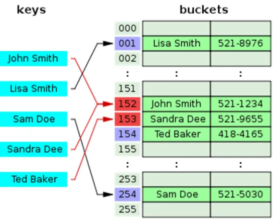
The hash table data structure is used to store and map key value pairs. This sort of data structure is also referred to as an associative array. With this data structure it is possible to directly refer to data sets in a table by the use of arithmetical transformations converting keys into table addresses. If ∈ 1, 2. . then one can store a set of data with a = in the table at the position with an = . With this simple method, the key value is directly used as pointer to the associated value. Sedgwick (1992) describes hashing to be a generalisation of the above outlined simple method for searching algorithms where such specific knowledge on the key is not available. The first step in the process of searching by the use of hashing is to find a suitable hash function which transforms the key into a table address. In the ideal case the hash function transforms different keys into different table addresses. In most of the cases the hash function will not be perfect and therefore it will transform more than one key into the same table address. Thus the second step in the process of searching by the use of hashing will be concerned with collision resolution.

3.4.2 The hash function

It is essential to find the right hash function and an effective implementation algorithm to achieve good hashtable performance. This could be quite a difficult task to achieve. As Wikipedia (2013), Rahm (2013) and University of Paderborn (2006) are describing it is a basic requirement for a hash function to uniformly distribute the hashvalues. If the hash values are not distributed uniformly, the number of collisions and the cost for their resolution will increase. To ensure uniformity by design the function may be tested empirically by the use of statistical tests.

(34)

3.4.3 Hash table statistics

The crucial factor of a hash table is the load factor α. It is calculated as follows: =

where n is the number of entries and m is the number of places or buckets in the hash table. The load factor should stay below a certain value for the hash table to perform well. On the other hand it is not of great use to bring it near 0 which means that memory is wasted.

3.4.4 Collision resolution

As in most cases the hash function will not be perfect. Collision resolution has to be considered. There are various approaches to this. Below different ways of collision resolution are described. Each of these is more suited for a specific type of data.

3.4.4.1 Separate chaining

The variant of collision resolution known as separate chaining implements each bucket as an independent entity with a list of entries stored. The cost of operation on such a hash table is: = + where = !"#$.

(35)

[image:35.595.107.431.119.317.2]

3.4.4.2 Separate chaining with linked lists

Figure 3.4-1: Hash collision resolved by separate chaining (Wikipedia)

(36)

3.4.4.3 Separate chaining with list heads

Figure 3.4-2: Hash collision by separate chaining with head records in the bucket array (Wikipedia)

Another type of collision resolution described by Wikipedia (2013) is the separate chaining with list heads. The first entry of each chain is stored in the bucket itself. Thus one pointer traversal can be saved in most cases. Cache efficiency of the hash table increases by the use of this solution.

[image:36.595.107.379.504.722.2]

3.4.4.4 Open addressing

(37)

Collision resolving by the use of open addressing means that every entry is stored in the bucket array itself. If some new data has to be inserted the system looks for free buckets. If the targeted bucket is already taken algorithms are used to search for the next free bucket where the entry will then be made. If a key is searched for, the same algorithms are used to scan through the buckets until either the entry is found or an empty bucket appears which indicates that the hash table does not contain the key searched for. The term “open addressing” underlines the basic concept that a place where an item is stored is not directly deducible from its hash value.

There are several algorithms used to store data in the hash table.

Name Description

Linear probing Fixed interval between probes (usually 1)

Quadratic probing The interval between probes is increased by adding the consecutive outputs of a quadratic polynomial to the originally calculated hash value

Double hashing The interval is calculated by another hash function

Table 3.4-1: Probing algorithms for open addressing

(38)

Figure 3.4-4: This graph compares the average number of cache misses required to look up elements

in tables with chaining and linear probing (Wikipedia)

(39)

3.4.5 Tree’s

The tree data structure used in this investigation is a means to display hierarchical lists. The Qt-Framework provides a class which implements such a tree. This class is called QTreeView and it is part of Qt’s model / view framework.

Figure 3.4-5: Qt model / view architecture

The model / view concept originates from the Smalltalk programming language and it is used to separate the data from its presentation, called the view.

(40)

Chapter 4:

Implementation

4.1

Introduction

As described in Chapter 1: Introduction a wholly new approach of how a project in the field of building automation is set up and realised is introduced by this investigation. The introduced approach is a paradigm change compared to the traditional approach. The bottom up approach (see Figure 1.1-1: Traditional approach) is changed into a top down approach (see Figure 1.2-1: New approach). The new approach orients itself on the object orientated paradigm well known from high level programming languages as C++, Stroustrup (2000). Furthermore it is based on the graphical programming languages known from the IEC 61131-3 Standard, IEC (2003).

4.2

Initial position

Some of the principles regarding SCADA-Systems used in this investigation are in use since 1999 by MST Systemtechnik AG in their SCADA-System called ProMoS NT, MST Systemtechnik AG (2013). The results of this investigation initially were planned to be an improvement to the current code generation system implemented in PromoS NT.

[image:40.595.99.554.495.735.2]

4.2.1 Template object concept

(41)

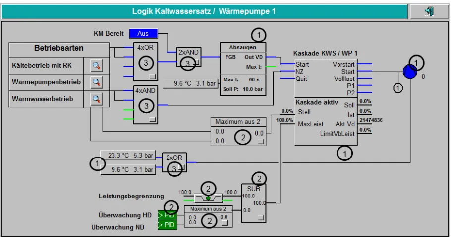
Figure 4.2-1: Logical plant diagram shows a typical Plant-Diagram used to program a heat-pump-system. In the table below the different elements, called TO (Template Objects) will be described.

Number Description

1 Highly sophisticated templates from a library for refrigeration applications

2 Templates from the standard template library

3 Templates to do logical connections

Table 4.2-1: Description of the TO

The TO concept is derived from the class concept well known in high level programming languages as C++, Stroustrup (2000). With the TO concept often used plant functions are encapsulated, an interface to access the public member functions, the graphic icon, and the necessary user interfaces are designed.

TO-Part Description

IL-Code PLC software

Graphic Icon Graphical representation for the TO in the plant diagrams (see Figure 4.2-1: Logical plant diagram (runtime mode))

1..n

User Interface(s)

A means for the user to interact with the TO.

Generator Template Used by the code generator to generate the function block calls.

Table 4.2-2: Parts of a TO

Well designed, tested and documented TO or even whole TO Libraries can accelerate the engineering process dramatically. Huge portions of PLC code can be reused in a wide range of projects.

(42)

4.2.2 Programming on the plant diagram

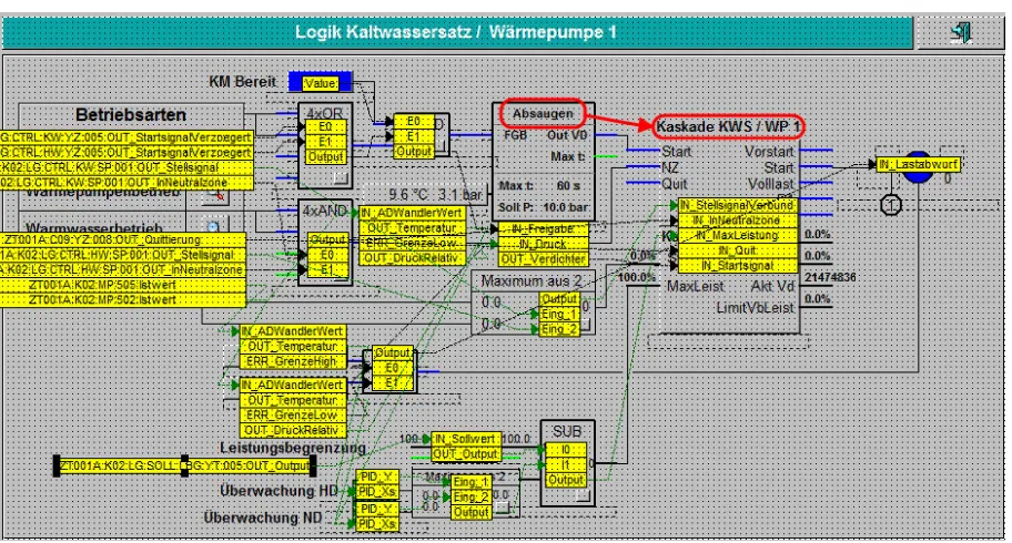
[image:42.595.100.554.150.391.2]

Currently there already is a way to do the connections on the plant diagram. To link a certain output of a TO to an input of another TO one has to switch from runtime mode to programming mode.

Figure 4.2-2: Logical plant diagram (programming mode)

As an example the WARN_Absaugzeit Signal of the Absaugen TO should be linked to the IN_ManuellMinus Signal of the Kaskade KWS / WP 1 TO.

[image:42.595.100.556.472.717.2]

(43)

[image:43.595.102.554.131.371.2]

To link these two signals together the first step is to click on the source TO (Absaugen) and to choose the desired output signal (WARN_Absaugzeit) from the appearing list.

Figure 4.2-4: Logical plant diagram (choose output signal)

After the desired signal has been chosen the second step is to click on the target TO (Kaskade KWS / WP 1) and to choose the desired input signal (IN_ManuellMinus) from the appearing list.

[image:43.595.99.555.477.714.2]

(44)

[image:44.595.100.556.87.330.2]

After the input signal is chosen the two signals are linked.

Figure 4.2-6: Logical plant diagram (signals linked)

The colouring of the link lines can be changed by the user. For the above example the colouring is described in the table below:

Colour Description

Black Link-type is a binary signal with state 0

light-green Link-type is a binary signal with state 1

dark-green Link-type is an analogue signal

Table 4.2-3: Colouring of the link lines

The connection established in the above example will result in the following line of generated IL (Instruction List) code:

;******************************************************************************

PB PBscoKaskade ; Manage scoKaskade-Objects

; Kaskade KWS / WP 1 [ZT001A:K02:LG:FGB:YZ:006]

(45)

STH F __frame.fNull ; IN-PAR

OUT F K02.LG.FGB.YZ_006.IN_BetrArtLokal

STH F K02.LG.FGB.YZ_008.WARN_Absaugzeit ; IN-PAR

OUT F K02.LG.FGB.YZ_006.IN_ManuellMinus

STH F K02.LG.FGB.YZ_002.Output ; IN-PAR Verknüpfung Neutralzone Leistungsregler OUT F K02.LG.FGB.YZ_006.IN_InNeutralzone

COPY R K02.LG.LAW.CL_001.Output ; IN-PAR Berechnung maximale Leistung R K02.LG.FGB.YZ_006.IN_MaxLeistung

STH F C09.YZ_008.OUT_Quittierung ; IN-PAR Signalisation OUT F K02.LG.FGB.YZ_006.IN_Quit

STH F K02.LG.FGB.YZ_008.OUT_Verdichter ; IN-PAR Absaugsteuerung OUT F K02.LG.FGB.YZ_006.IN_Startsignal

COPY R K02.LG.FGB.YZ_005.Output ; IN-PAR Maximalauswahl Stellgrösse R K02.LG.FGB.YZ_006.IN_StellsignalVerbund

CFB scoKaskade ; Scheco Kaskaden-Modul zur Verdichter-Freigabe DB 4013 ; [=01] CFG_AnzVd

F __frame.fNull ; [=02] CFG_KkTyp F 1440 ; [=03] ERR_AlarmP1 F 1441 ; [=04] ERR_AlarmP2

F C09.YZ_008.OUT_Quittierung ; [=05] HW_QuitEing F 1737 ; [=06] IN_BetrArtLokal

F 1747 ; [=07] IN_InNeutralzone F 1749 ; [=08] IN_ManuellMinus F 1750 ; [=09] IN_ManuellPlus R 1509 ; [=10] IN_MaxLeistung R 1510 ; [=11] IN_Modus F 1755 ; [=12] IN_Quit F 1761 ; [=13] IN_Startsignal

(46)

F 1800 ; [=16] OUT_DelayOn R 1572 ; [=17] OUT_IstLeist

R 1584 ; [=18] OUT_pDbRemVdRec R 1585 ; [=19] OUT_pDbRemVdSend R 1591 ; [=20] OUT_Sollleist

R 2148 ; [=21] OUT_TotalVbLeistung F 1830 ; [=22] OUT_VerbundEin F 1832 ; [=23] OUT_Volllast DB __PDB+8 ; [=24] Datablock DB __PDB+9 ; [=25] Datablock[8] DB __PDB+17 ; [=26] Datablock[8] DB __PDB+25 ; [=27] Datablock[8]

EPB ; End Programblock scoKaskade

;******************************************************************************

Listing 4.2-1: Generated Function Block call with parameters

4.3

Current logical template objects

In Figure 4.2-1: Logical plant diagram (runtime mode) LTO (Logical TO) can be seen (also see Table 4.2-1: Description of the TO line 3). These are the logical TO used at the moment.

LTO Name Description

AND02 AND gating with two inputs

AND04 AND gating with four inputs

ORH02 OR gating with two inputs

ORH04 OR gating with four inputs

Table 4.3-1: Current LTO

(47)

applies input and output resources for each instance used. The current implementation also contains some engineering inconveniences. If one needs to increase the number of used inputs on a LTO where all inputs are already in use, an additional LTO is needed or, in case the maxed LTO is one with only two inputs, the LTO has to be changed. The same process takes place if the digital technology function has to be changed. This slows the engineering process significantly. To avoid this, the basic digital technology functions (AND, OR) have to be available as one logic TO with up to ten inputs with the possibility to alter the digital technology function at runtime.

In the life cycle of a project the dependencies of an input parameter can change. To make a program modification as simple as possible, the number of used input parameters of a logical TO should be easy to increment or decrement respectively. It should be possible to easily add or remove connections and afterwards download the edited program to the running PLC. To realize this and to make the programming of a facility on the plant diagram more efficient, the logic template object is necessary. One possible solution of an implementation of such a template object on a PLC-System of Saia-Burgess is shown in the following section. The template objects can be modelled according to the UML 2.0 standard Kecher (2006). Some attempts have been made to use UML to generate PLC code similar to Sacha (2005) and Lee et al. (2002) but have been abandoned because it is not in the scope of this investigation.

4.4

System design

As can be derived from the objectives in Chapter 1.3 Objectives the LTO will be run on a virtual machine. This is a completely new approach. On PLC-Systems from Saia-Burgess due to compatibility reasons the PLC software also runs on a virtual machine. This fact ensures the usability, reusability of existing software on new hardware. Only the software libraries have to be updated and the software has to be compiled for the new target hardware to reuse the software of an existing plant while migrating to a new hardware generation.

(48)

4.4.1 System overview

Figure 4.4-1: System overview

4.4.2 Storage of the data

The connection data is stored in appropriate data structures. The data structure used depends on the PLC-System. For this investigation, PLC-Systems from Saia-Burgess are used exclusively. On Saia-Burgess PLC-Systems, data blocks are used to store the generated code. A data block is a one-dimensional array, consisting of 32-bit registers. The data type usually used with data blocks is DWU (Double Word Unsigned). 7999 data blocks are available with up to 16384 32-bit registers.

The data blocks from 0 up to 3999 can only store 383 32-bit values. Because of hardware reasons the access to these data blocks is significantly slower than to the ones in the higher memory area. For this reason, the data blocks starting from 4000 are used.

4.5

Virtual machine on the PLC-System

(49)

virtual machine deals with one single task. This is also true for the virtual machine developed in this investigation.

4.5.1 Process virtual machine

A case in point for a process virtual machine is the java vm. The byte code produced by the java language processor is interpreted in the virtual machine as a single process. The source code can be interpreted in different ways, Smith &Nair (2005).

• Decode-and-dispatch interpretation • Indirect threaded interpretation

• Predecoding and direct threaded interpretation • Binary translation

For the implementation on a PLC-System only the first and second type are of importance because no transformation from one ISA (Instruction Set Architecture) into another is made. Below these two types are discussed.

4.5.2 Decode and dispatch Interpretation

A decode and dispatch interpreter is structured around a central loop that decodes an instruction and then dispatches it to an interpreter routine based on the type of instruction. This kind of interpretation involves a lot of branches, which can be a very time consuming task. There is an interpreter routine for every source instruction.

(50)

4.5.3 Indirect threaded interpretation

In the indirect threaded interpreter the central loop is omitted (see Figure 4.5-1; Decode and dispatch interpretation). To every interpreter routine the necessary code to fetch and dispatch the next instruction is added.

Figure 4.5-2: Indirect threaded Interpretation

4.5.4 Chosen type of virtual machine

For this investigation, the decode and dispatch interpretation is used. The solution implemented uses the ideas of this type of virtual machine. It has to be adapted to the needs of PLC-Systems. The interpreter routines are implemented as functional blocks according to the IEC 61131-3 norm, IEC (2003).

(51)

4.5.5 Design of the virtual machine

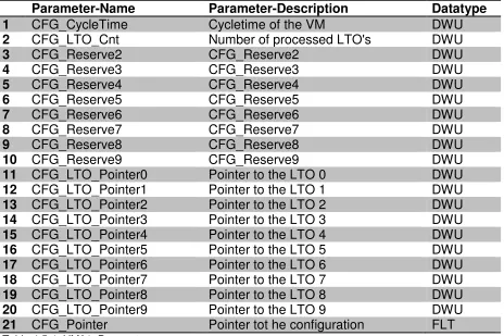
The virtual machine has been developed as a TO. It is called VM001. The VM001 TO consists of 21 parameters.

Parameter-Name Parameter-Description Datatype

1 CFG_CycleTime Cycletime of the VM DWU

2 CFG_LTO_Cnt Number of processed LTO's DWU

3 CFG_Reserve2 CFG_Reserve2 DWU

11 CFG_LTO_Pointer0 Pointer to the LTO 0 DWU

[image:51.595.97.561.153.462.2]

21 CFG_Pointer Pointer tot he configuration FLT

Table 4.5-1: VM01: Parameters

• Parameters 1 to 10 are used for configuration purposes or are reserved for future development.

• Parameters 11 to 20 are used to store the pointers to the configuration data blocks of the LTOs processed by the VM001 TO. By means of these pointers the VM001 TO can fetch the necessary data from the LTO linked to it. All configuration data and the LTO link information are stored in the configuration data block of the VM001 TO.

(52)

4.5.6 Implementation of VM001

The VM001 TO acts as a decode and dispatch loop in the system. To simplify the implementation the interpreter routines are placed in a separate library file, VMLib.src (also see Appendix B Source code VMLib.src).

4.6

The new logical template object

A new LTO (Logical Template Object), the LTO01, has been developed to remove the above discussed disadvantages. With the newly developed LTO it is possible to change the digital technology function at runtime and the number of inputs has been increased to ten. Of course this increased number of inputs does not completely remove the possibility of running out of unused inputs but it minimises it. In the following section the LTO01 TO is outlined in depth.

4.6.1 Design of the LTO01

The basic design can be seen in the table below.

Parameter-Name Parameter-Description Datatype

1 CFG_Function Logical function DWU

2 CFG_NbrOfUsedInputs Number of used Inputs DWU

11 CFG_AddressInput0 Addresse input 0 DWU

21 CFG_LogicInput0 Logic of input 0 DWU

(53)

31 CFG_AddressOutput Addresse output DWU

32 CFG_AddressOutputInvers Addresse invers output DWU

33 IN_Input0 Logical input 0 BIT

43 OUT_Output Output of LTO BIT

44 OUT_OutputInvers Invers output of LTO BIT

[image:53.595.89.558.69.337.2]

45 CFG_Pointer Pointer tot he configuration FLT

Table 4.6-1: LTO01: Parameters

The LTO01 TO acts as a container for the data used by the VM001 TO. In the whole system the LTO01 TO represents the source code which in turn represents the plant logic. For the design of the new LTO some fundamental changes have been made to reduce the cost of resources. In the old LTO the input signals use their own PLC resources which are binary signals, called flags in Saia-Burgess PLC-Systems. As can be seen in Chapter 4.2.2 Programming on the plant diagram a binary conjunction results in the following line of IL code:

STH F K02.LG.FGB.YZ_008.WARN_Absaugzeit ; IN-PAR OUT F K02.LG.FGB.YZ_006.IN_ManuellMinus

Listing 4.6-1: Generated IL code for a binary conjunction

(54)

TO A

Binary output signal

LTO B

Binary input signal STH F output signal

OUT F input signal

TO A

Binary output signal pointer = Binary input signal pointer

LTO B

Figure 4.6-1: Reduce cost of binary resources

The LTO01 TO implements the above mentioned concept to reduce the cost of binary resources. The input signals are simple containers for the pointers to the particular output signals.

All configuration data is stored in a datablock (see Table 4.6-1: LTO01: Parameters). • Parameters 1 to 10 are used for configuration purposes or are reserved for

future development.

• Parameters 11 to 20 are used to store the input pointers to the appropriate output signals.

• Parameters 21 to 30 contain the information which binary state of the respective input signal is to be used.

• Parameters 31 and 32 hold the pointers to the output signal and to the inverted output signal respectively.

• Parameters 33 to 42 are the containers for the input pointers.

• Parameters 43 and 44 are the real output signals which can be used to establish conjunctions to other TO.

(55)

4.6.2 Implementation of LTO01

At the moment the LTO01 executes two basic digital technology functions. These are the AND-Function and the OR-Function. For each one of the ten input signals the used binary state can be adjusted by the values stored in parameters 21 to 30 of the configuration data block. The digital technology function and the number of input signals used can be parameterised with parameter 1 and 2 of the configuration data block. The LTO01 requires the programmer to use the input signals in sequence starting from input signal 1 to 10 to allow for the possibility of changing the number of used input signals at runtime.

4.7

Implemenation of the interpreter routines

As mentioned above, 4.5.6 Implementation of VM001, to keep the VM001 as simple as possible, the interpreter routines have been implemented in a separate library file (also see Appendix B Source code VMLib.src). For each implemented digital technology function a function block has been developed. A uniform interface has been designed for the function blocks.

4.7.1 Functionblock interface fbAnd

; ***************** Function: AND ******************* ; ***************** Functionblock *******************

FB fbAnd ; Call Function AND rLtoAddress DEF = 1 ; Pointer to the actual LTO

rInputAddresses DEF = 2 ; Pointer to the input addresses of the actual LTO rInputLogics DEF = 3 ; Pointer to the input logic's of the actual LTO rOutputAddresses DEF = 4 ; Pointer to the output addresses of the actual LTO

Listing 4.7-1: Functionblock interface fbAnd

4.7.2 Functionblock interface fbOr

; ***************** Function: OR ******************** ; ***************** Functionblock *******************

(56)

Listing 4.7-2: Functionblock interface fbOr

4.7.3 Functionblock interface fbXor (skeleton only)

; ***************** Function: XOR ******************* ; ***************** Functionblock *******************

FB fbXor ; Call Function XOR rLtoAddress DEF = 1 ; Pointer to the actual LTO

Listing 4.7-3: Functionblock interface fbXor

4.7.4 Real local variables (temporary data)

To minimise the cost of resources a new feature using real local variables has been extensively applied. The temporary data has to be defined inside the block which is using them. As it is common practice with local variables in high level languages as C++, the variable exists only inside this block. The type of block is irrelevant for the behaviour of the temporary data.

; **************** Local Variables ***************** FUNCTION_OR_LOCALS:

fInputs TEQU F [10] ; Temporary Flags

fLogics TEQU F [10] ; Temporary Flags

fInputsLinked TEQU F [10] ; Temporary Flags

fHfOutput TEQU F ; Temporary Flag

fTempLogic TEQU F ; Temporary Flag

rInputCount TEQU R ; Temporary Register

rHrLtoAddress TEQU R ; Temporary Register rSaveTempIndex TEQU R ; Temporary Register rSaveInputAdresses TEQU R ; Temporary Register rSaveInputLogics TEQU R ; Temporary Register FUNCTION_OR_END_LOCALS:

; **************** Local Variables *****************

(57)

4.7.5 Get the number of used inputs

By means of the first parameter of the functionblock, rLtoAddress (see 4.7.1 Functionblock interface fbAnd) the interpreter routine accesses the configuration data of the according LTO and gets the number of used inputs. To access the LTO data block a firmware function call is made (CSF; Call Special Function).

; **************** Get Input Count ****************** FUNCTION_AND_GET_CNT:

COPY rLtoAddress ; Copy lto-address rHrLtoAddress ; to helper register CSF S.SF.DBLIB.Library ; Library number

S.SF.DBLIB.GetDBItem ; Read a single DB item

rHrLtoAddress ; 1 R|K IN, DB number (any DB number)

1 ; 2 R|K IN, DB item

rInputCount ; 3 R OUT, Value read SUB rInputCount ; Subtract from InputCount

1 ; the constant 1

rInputCount ; and save the value

FUNCTION_AND_END_GET_CNT:

; ************* End Get Input Count *****************

Listing 4.7-5: Get input count

4.7.6 Process the digital technology function

The processing of the digital technology functions is making heavy use of the index register of the Saia-Burgess PLC-System. In a first step the different indexes are created and saved.

; **************** Process function ***************** FUNCTION_AND_PROCESS:

; ********** Get Inputs

SEI 0 ; Set index to 0

STI rSaveTempIndex ; save index

SEI rInputAddresses ; Set index register to the base adresse of the input STI rSaveInputAdresses ; save index

SEI rInputLogics ; Set index register to the base adresse of the input-logics STI rSaveInputLogics ; save index

Listing 4.7-6: Prepare indexes

In the second step the state of the input is checked and saved to a temporary flag.

(58)

RSI rSaveInputAdresses ; restore index

STHX F 0 ; If input is high

RSI rSaveTempIndex ; restore index OUTX fInputs ; set flag to high too

Listing 4.7-7: Check state of the input

In the third step the information which binary state of the input should be used in the conjunction is retrieved.

; ********** Get Logics

FUNCTION_AND_LOGIC_LOOP:

RSI rSaveInputLogics ; restore index

BITOX 1 ; Get one bit

R 0 ; out of the register

F fTempLogic ; onto the flag STI rSaveInputLogics ; save index

RSI rSaveTempIndex ; restore index

STH fTempLogic ; if temporary flag is high

OUTX fLogics ; set flag to high too

RSI rSaveInputLogics ; restore index

INI 8191 ; increment index

STI rSaveInputLogics ; save index

RSI rSaveTempIndex ; restore index

INI rInputCount ; increment index

GETX rInputAddresses ; copy address of next input rSaveInputAdresses ; to register

JR H FUNCTION_AND_INPUT_LOOP ; jump to loop if there are more inputs

Listing 4.7-8: Get logic information

(59)

A B Y (' ∶= ) * +)

0 0 0

0 1 1

1 0 1

[image:59.595.94.243.70.176.2]

1 1 0

Table 4.7-1: Truth table for the XOR-Function

A := State of the input signal

B := State of the configuration signal

Y := Result of the XOR function and used state in the conjunction

; ********** Link input-logic

FUNCTION_AND_INPUTLOGIC_LOOP:

STHX fInputs ; Link inputs

XORX fLogics ; with logic

OUTX fInputsLinked ; and save it to a new array

JR H FUNCTION_AND_INPUTLOGIC_LOOP; jump to loop if more inputs to link

Listing 4.7-9: Calculate the binary state used in the conjunction

In the fifth step the processing of the digital technology function is done.

; ********** Process function

ACC H ; Set accu to high state

SET fHfOutput ; Set helper flag to high state FUNCTION_AND_FUNCTION_LOOP:

STH fHfOutput ; Link the state of the helper flag with the ANHX fInputsLinked ; state of the linked input

OUT fHfOutput ; set the helper flag to the state of the input

JR H FUNCTION_AND_FUNCTION_LOOP; jump to loop if more inputs to check

(60)

In the sixth and last step of the interpreter routine, the output signals of the LTO are set accordingly to the result of the conjunction.

; ********** Set outputs

SEI rOutputAddresses ; Set index to the base address of the output array

STH fHfOutput ; If the