Vegetative Rhombic Pattern Formation Driven by Root Suction for an Interaction Diffusion Plant Ground Water Model System in an Arid Flat Environment

http://dx.doi.org/10.4236/ajps.2015.68129

Vegetative Rhombic Pattern Formation

Driven by Root Suction for an

Interaction-Diffusion Plant-Ground Water

Model System in an Arid Flat Environment

Inthira Chaiya

1

, David J. Wollkind

2

, Richard A. Cangelosi

3

, Bonni J. Kealy-Dichone

3

,

Chontita Rattanakul

1

1_{Department of Mathematics, Faculty of Science, Mahidol University, Bangkok, Thailand} 2_{Department of Mathematics, Washington State University, Pullman, USA}

3_{Department of Mathematics, Gonzaga University, Spokane, USA} Email: [email protected]

Received 26 March 2015; accepted 25 May 2015; published 28 May 2015

Copyright © 2015 by authors and Scientific Research Publishing Inc.

This work is licensed under the Creative Commons Attribution International License (CC BY).

http://creativecommons.org/licenses/by/4.0/

Abstract

A rhombic planform nonlinear cross-diffusive instability analysis is applied to a particular inte-raction-diffusion plant-ground water model system in an arid flat environment. This model con-tains a plant root suction effect as a cross-diffusion term in the ground water equation. In addition a threshold-dependent paradigm that differs from the usually employed implicit zero-threshold methodology is introduced to interpret stable rhombic patterns. These patterns are driven by root suction since the plant equation does not yield the required positive feedback necessary for the generation of standard Turing-type self-diffusive instabilities. The results of that analysis can be represented by plots in a root suction coefficient versus rainfall rate dimensionless parameter space. From those plots regions corresponding to bare ground and vegetative patterns consisting of isolated patches, rhombic arrays of pseudo spots or gaps separated by an intermediate rectan-gular state, and homogeneous distributions from low to high density may be identified in this pa-rameter space. Then, a morphological sequence of stable vegetative states is produced upon tra-versing an experimentally-determined root suction characteristic curve as a function of rainfall through these regions. Finally, that predicted sequence along a rainfall gradient is compared with observational evidence relevant to the occurrence of leopard bush, pearled bush, or labyrinthine tiger bush vegetative patterns, used to motivate an aridity classification scheme, and placed in the context of some recent biological nonlinear pattern formation studies.

Keywords

Threshold-Dependent Pattern Formation

1. Introduction

von Hardenberg et al.[1] devised a plant-ground water (sometimes called soil water) interaction-diffusion sys-tem to model self-organized vegetative pattern formation in arid environments (reviewed by Rietkerk et al. [2]). Here the positive feedback for an activator consumer (e.g., plants) in the plant equation and the self-diffusivity advantage for an inhibitory limiting resource (e.g., ground water) provided the necessary conditions for the onset of Turing [3] pattern formation. von Hardenberg et al.’s [1] model also included the effect of plant root suction by adding a cross-diffusion term in their ground water equation. Rietkerk et al.[4] performed numerical simula-tions using reflecting boundary condisimula-tions on a similar interaction-diffusion model system consisting of three partial differential equations describing the spatio-temporal behavior of plant density, soil water, and surface water, respectively, but excluding the root suction cross-diffusion term in their soil water equation. That model had been carefully developed by HilleRisLambers et al.[5] for a flat semi-arid grazing system.

We wish to formulate an interaction-diffusion model system for N X Y

(

, ,

τ

)

≡ plant biomass density (gm/m2) and W X Y

(

, ,

τ

)

≡ ground (soil) water content (mm of depth), where

(

X Y,

)

≡ two-dimensional coordinate system (m, m) and

τ

≡

time (d), based upon the interaction terms of Rietkerk et al. [4] and the diffusion terms of von Hardenberg et al. [1], defined on a flat unbounded arid environment. Toward that end, we first introduce the auxiliary dependent variable O X Y

(

, ,

τ

)

≡ surface water content (mm of depth) and the coupled interaction- diffusion model system given by

( ) ( ) ( ) ( ) ( ) ( )

2 , 2 , 2 ,

N W W O O

N

N W

Q Q O Q

τ τ τ

∂ ∂ ∂

− ∇ ⋅ − ∇ ⋅ − ∇

= =

∂ J ∂ J ∂ = ⋅J (1.1)

where ([1] [4])

( ) ( ) 2 ( ) 2

1 2 1 2

, ,

,

N M W M

M

O

M

cg N k g N k

Q dN Q i rW Q R i

W k N

WN f WN f

O

W k O N k

k

+ +

= − = − − = −

+ + + + (1.2)

( ) ( )

₍

₎

( )

2 , 2 , 2 ,

N W O

N N DW N DO

D ∇ ∇ W ρ O

= − = − − = − ∇

J J J (1.3)

with ∇ ≡ ∂ ∂ ∂ ∂2

(

X, Y

)

and ∇ ⋅2 J=

(

∂J1 ∂ ∂X, J2 ∂Y

)

for J=

(

J1,J2

)

. Here gM ≡ maximum specific

water uptake rate by the plants,

c

≡

conversion of water uptake by the plants to plant growth, d≡ specific loss rate of plant density due to mortality, k₁≡ half-saturation soil water constant relevant to specific plant growth and water uptake, r≡ specific loss rate of soil water due to evaporation and drainage, R≡ rainfall rate, i_M ≡ maximum specific water infiltration rate, k₂≡ plant saturation shaping constant for water infiltra-tion , f ≡ fraction of maximum specific water infiltration rate in the absence of plants, D_N ≡ dispersal coef-ficient for plants, D_W ≡ diffusion coefficient for ground water, D_O ≡ diffusion coefficient for surface water,

S

D ≡ coefficient of plant root suction, and ρ =D_S D_W .

More than forty years ago, Keller and Segel [6] proposed the initiation of slime mold aggregation viewed as an instability in a landmark paper with that title. They formulated a mathematical reaction-diffusion model sys-tem for the aggregation of the cellular slime mold Dictyosteliumdiscoideum involving four dependent variables: Namely, the density of this amoeba; the concentrations of the acrasin and acrasinase produced by it which me-diate its aggregation; and the concentration of an intermeme-diate complex formed by these chemicals in a reversi-ble reaction. Keller and Segel [6] then simplified that model to a two-component system involving just the den-sity of the amoeba and the concentration of the acrasin by making Haldane’s assumption that the complex was in chemical equilibrium and the additional assumption that the total concentration of the acrasinase enzyme in both its free and bound state was a constant. This simplified model included flux terms deduced from Fickian self-diffusion of its two components and a chemotaxis term for the amoeba generated by the introduction of cross-diffusion involving the acrasin gradient.

our model system (1.1)-(1.2)-(1.3) by assuming that the surface water is in hydrological equilibrium and making the quasi stationary approximation that

( ) 2

2

0 M .

O N k f

R i O

N Q

k + ≡ ⇒ =

+ (1.4) Such an assumption is dependent upon D_O being relatively much greater than either D_W or D_N and O having a much faster time scale than either W or N [4].

Then, introducing (1.4) into (1.1)-(1.2)-(1.3) by replacing the rate of infiltration term in Q( )W with R, we obtain the final formulation of our interaction-diffusion plant-ground water model system

(

)

2

(

)

(

2 2

)

2 , 2 2

, _N , _W

N W

F N W D N G N W D W ρ N

τ τ

∂ _∇ ∂ _{= + ∇ − ∇}

∂ = + ∂ (1.5)

where

(

)

(

)

2

2 2 2

1 1

, , , W .

, cgM gM

F N W WN dN G N R rW

W k W k

WN

= − = −

≡

+

∇ ∇ −

+

∇ ⋅ (1.6)

Our main purpose in doing so is to devise a model system of this sort that demonstrates root suction alone can generate the two-dimensional vegetative patterns (e.g., leopard bush, pearled bush, and labyrinthine tiger bush) occurring in arid flat environments as described by Rietkerk et al. [2]).

2. Equilibrium Points and Their Linear Stability

There exist two equilibrium points of model system (1.5)

0, 0

N

N≡ W ≡W (2.1) satisfying

(

0, 0

)

(

0, 0

)

0

F N W =G N W = (2.2) given by

0 0, 0 ;

N = W =R r (2.3) and

(

)

(

)

(

)

0 Ne 1 1 , 0 We k1 1 with c M .

N = = c d _R−rk δ− _ W = = δ− δ = g d (2.4) Note that (2.3) which exists for all parameter values corresponds to a bare ground or no vegetation situation while (2.4) which only exists for N We, e >0 or, equivalently,

1

1 rk R,

δ > + (2.5) corresponds to a community equilibrium point or a state exhibiting a nontrivial homogenous vegetative distribu-tion. In this context, we adopt the far-field condition that

2 2 remain bound

, ed as X .

N W +Y → ∞ (2.6) We next wish to examine the linear stability behavior of these critical points and shall proceed sequentially. That is we begin with (2.3) by considering a separation of variables solution to system (1.5) and boundary con-dition (2.6) of the form

(

)

(

)

( )

2

1 11 1

, , 0 cos e O ,

N X Y τ = +ε N QX Στ + ε (2.7)

(

)

(

)

( )

2

1 11 1

, , cos e O ,

W X Y τ =R r+εW QX Στ + ε (2.8)

2 2

1 1, N11 W11 0, Q 0,

ε

_ + ≠ ≥ (2.9) and find that

(

)

(

)

2 2

1 δ 1 R−rk1 R+rk1 −DNQ ro 2 r D Qw .

Upon examination of (2.10) it follows that Σ <₂ 0 identically and Σ <₁ 0 provided

1

1 rk R

δ < + (2.11) Hence we can conclude that (2.11) represents the linear stability criterion for this bare ground equilibrium point. Since the community equilibrium point of (2.4) does not exist for these parameter values by virtue of (2.5), an exchange of stabilities between the two critical points of system (1.5) occurs at δ = +1 rk R₁ .

The primary focus of our research is on the stability behavior of this community equilibrium point. Now in-troducing the nondimensional variables and parameters

(

) (

) (

1 2

)

, W , , , e, e,

x y = d D X Y t=τd n=N N w=W W (2.12)

(

)

1

( )

1 ,

, 1 R rk k N W, ,

r d d D D c

γ = α=_δ − − _ µ= β = ρ (2.13) we transform system (1.5) and far-field condition (2.6) into

(

)

2

(

)

2 2

, , , ,

n w

n w

n w

t w n

t µ n αβ

∂ _{Θ ∇} ∂ _{Ψ ∇ − ∇}

∂ = + ∂ = + (2.14)

where ∇ ≡ ∂ ∂ + ∂ ∂2 2 x2 2 y2,

(

)

(

)

(

)

1 1

, , , 1 ,

n w w n n w w wn

w w

n

δ _{α γ} αδ

δ δ

= − = + − −

− +

Θ Ψ

−

+ (2.15)

and

2 2

remain bound

, ed as x .

nw +y → ∞ (2.16) Observe that the equilibrium point in question corresponds to

1

n= ≡w (2.17) in our dimensionless formulation since

( )

1,1 =

( )

1,1 0.

Θ Ψ = (2.18) Here we are concerned with the stability of this solution to initially infinitesimal one-dimensional perturba-tions. Toward that end, we consider a reduced form of our basic system with 2 2 2

x

∇ ≡ ∂ ∂ ; seek a separation of variables solution to it satisfying

( )

( )

( )

2

( )

( )

( )

2

1 11 1 1 11 1

, 1 cos e t O , , 1 cos e t O

n x t = +εn qx σ + ε w x t = +εw qx σ + ε (2.19)

where

q

≥

0

and

σ

are the wavenumber and growth rate of the linear perturbation quantities (i.e. ε₁ 1)

with n₁₁2 +w₁₁2 ≠0 for the constants n₁₁ and w₁₁; and obtain

(

2

)

2

(

)

2 4

(

)

2

01 01 01 01 10

1

;q q q q 0

σ =σ +_ +µ −ψ _σ µ+ − µψ +αβθ −θ ψ =

 (2.20)

where

( )

( )

1 1

1,1 , 1,1

! ! ! !

p s p s

ps p s ps p s

n w

p s w p s n

θ = ∂ + Θ ψ = ∂ + Ψ

∂ ∂ ∂ ∂ (2.21)

which are tabulated below for the relevant values of p and s.

Note that in (2.20) we have implicitly made use of the fact that θ =₁₀ 0. Upon substitution of these expansion coefficients fromTable 1 into (2.20), we obtain the explicit secular equation for

σ

(

)

(

)

2 2 4 2

0,

1 q q q

σ +_ +µ + + ∆γ α σ µ_ + +_µγ α µ β+ − ∆_ +α∆ = (2.22) where ∆ >0 for those

δ

satisfying (2.5). Thus, since quadratics of the form of (2.22) have roots with nega-tive real parts provided their coefficients are posinega-tive, we can conclude that the community equilibrium point is stable to linear homogeneous perturbations for which q2 =0. Further observe that in the absence of plant root suction (

β =

0

) this equilibrium point would be linearly stable to heterogeneous perturbations, for which

2

0

Table 1.Interaction expansion coefficients.

1 1 2

10 20 21 30 0, 01 11 1 , 02 12 , 03

θ ₌θ ₌θ ₌θ ₌ θ ₌θ _{= ∆ = −}δ− θ ₌θ _{= −∆}δ θ− _{= ∆}δ−

1 2

10 , 01 , 20 21 30 0, 02 12 , 03

ψ _{= −}α ψ _{= − − ∆}γ α ψ ₌ψ ₌ψ ₌ ψ ₌ψ _{= ∆}α δ− ψ _{= − ∆}α δ−

(

2

)

( )

2 2

( )

0 q ; , , , q 1q .

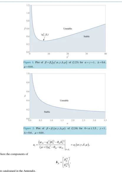
β β> α γ ∆ µ =_µ α∆ _ + +γµ α∆ +µ (2.23) For fixed

α

, γ, ∆, and µ, the curve

(

2

)

0 q ; , , ,

β β= α γ ∆ µ in the first quadrant of the 2

q −

β

plane is marginal since it serves as a boundary between the linearly stable region where 0≤ <β β₀

(

q2; , ,α γ ∆,µ

)

and the unstable region of (2.23). This marginal stability curve has a minimum point at

(

2

)

,

c c

q β given by

(

)

(

)( )

2

1 1

, 2 .

c c

q = ∆ µ α β = µ ∆ α + γµ ∆ α +µ

(0.1) Thus, when β β> _c there exists a band of squared wavenumbers q2 centered about qc2 corresponding to

growing disturbances for which σ >₀ 0 where σ₀ represents the most dangerous mode of (2.22) while when

c

β β< there exists no such band (see Figure 1).

The restriction of q2≡q_c2 in the expansions relevant to the weakly nonlinear stability analyses of the next three sections, allows us to consider

σ

₀=

σ β

_c

( )

, for fixed

α

, γ, µ and ∆, such that

σ β

c

( )

<0 when

c

β β< ,

σ β

c

( )

c =0 and σ βc

( )

>0 when β β> c (see Figure 1). Hence, the locus

β β α γ

= c

(

; , ,∆

µ

)

with

β α γ

c

(

; , ,∆

µ

)

defined by (2.24), is a marginal stability curve in the

α β

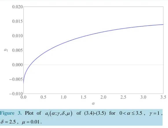
− plane, with γ, ∆, and µ fixed. We plot that locus inFigure 2 for 0<α≤3.5,

γ =

1

, ∆ =0.6, and

µ

=0.01, corresponding to the typical parameter values ([1] [4])

(

)

(

2

)

(

2

)

1

0.05 mm d gm m , 10 gm m mm , 0.2 d , 5 mm

M c d r

g = = = = k = (2.25)

( )

2 2

mm d 3 mm d , 0.1 m d , 10 m d .

2 3 < ≤R DN = DW = (2.26)

3. One-Dimensional Analysis: Stuart [7]-Watson [8] Nonlinear Stability Results

In the previous section we deduced the critical conditions for the occurrence of cross-diffusive instabilities when

0

α > . To ascertain both the long-time behavior and spatial pattern of such growing perturbations we must con-sider the nonlinear terms in our basic equations. Defining the vector quantities

( )

,

( )

_{( )}

, and , ,

jk jk

jk

n n x t

x y

w w x t

   

=    



  v = 

v (3.1)

it is standard operating procedure to examine the weakly nonlinear stability of our community equilibrium point by letting [9]

( )

( )

( )

2

( )

(

)

3

( )

( )

(

)

00 1 11 1 20 22 1 31 33

, ~ cos _c cos 2 _c cos _c cos 3 _c ,

x t +A t q x +A t _ + qx _+A t _ qx + q x _

v v v v v v v (3.2)

where n₀₀ =w₀₀ =1, and A t₁

( )

satisfies the amplitude equation 3 1

1 1 1 d

.

d ~ A

A

a A

t σ − (3.3) Then, the substitution of this solution into (2.14)-(2.15)-(2.16) and the expansion of its interaction terms in a Maclaurin series, yields six vector problems: The O(1) problem is satisfied identically given that n₀₀ =w₀₀ =1 are the components of the uniform homogeneous solution; the O

( )

A₁ problem is the same as the linear one of the previous section with q≡q_c, θ₀₁w₁₁=

(

σ θ− ₁₀+µq_c2

)

n₁₁, n₁₁=1, and

σ σ β

= _c

( )

; the solutions of the two _O

( )

_A12 _{problems are catalogued in the Appendix; of the two}

( )

3

1

O A problems, we are only concerned with the one proportional to cos

( )

q xc containing the Landau constant a1. Using the usual Fredholm

Figure 1. Plot of

(

2

)

0 q; , , ,

β β= α γ ∆µ of (2.23) for α γ= =1, ∆ =0.6, 0.01

µ = .

Figure 2. Plot of β β α γ= c

(

; , ,∆µ

)

of (2.24) for 0< ≤α 3.5, γ =1, 0.6

∆ = , µ =0.01.

(

)

( ) ( )

(

)

(

)

2

01 31 01 31

1 1

2

0 1

2

1 01

, ; , , 1

c

c c

b

a a

q

q b

β β

ψ θ

α γ δ µ

µ θ ψ

= −

= −

=

+ − − (3.4)

where the components of

( )

( )

1

2 , jk jk

jk

b

b

 

 

  =



b (3.5)

are catalogued in the Appendix.

The stability behavior of the Landau equation (3.3) is dependent upon the sign of a₁. Thus, to predict this behavior, we must analyze the formula for a₁

(

α γ δ µ

; , ,

)

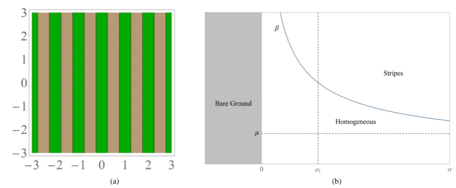
given by (3.4) with its interaction coefficients as listed in Table 1 and the components of (3.5) as defined in the Appendix. Hence we plot a₁

(

α γ δ µ

; , ,

)

in

[image:6.595.92.507.72.657.2]

Figure 3. Plot of a₁

(

α γ δ µ; , ,

)

of (3.4)-(3.5) for 0< ≤α 3.5, γ =1, 2.5

δ= , µ =0.01.

From Figure 3 we observe that a₁

(

α

;1, 2.5, 0.01

)

has a zero at α =0.172 such that

1 1

1 1

0 for 0 0.172,

0 for 0.172. a

a

α α

α α

< < < ≡ 

 > > ≡

 (3.6)

Given these conditions, we may conclude that there exist two supercritical cases when α α> ₁: Namely, for 0< <β βc, the community equilibrium point is stable, resulting in a uniform homogeneous vegetative

distribu-tion n x t

( )

, ~ 1; while for β β> _c, there occurs a re-equilibration producing stationary parallel vegetative stripes

( )

, ~ 1 ecos

(

2π c

)

n x t +A x

λ

(3.7) of amplitude A_e=

(

σ_c a₁

)

1 2 >0 and characteristic wavelength

(

)

1 2 2π 2 and

c qc c DW d c

λ ₌ λ∗ ₌ λ

(3.8) in dimensionless and dimensional variables, respectively. These supercritical stripes are plotted inFigure 4(a)

where regions of higher density

(

n>1

)

appear dark and those of lower density

(

n<1

)

appear light.

When 0< <α α₁ that bifurcation is subcritical and there also exist two cases: Namely, again, for 0< <β βc and β β> c, respectively. In general such subcritical behavior requires us to take into account

higher order terms in our expansions which can cause the development of a uniform homogeneous vegetative distribution and isolated local vegetative patches (see the last section for a detailed discussion of this topic).

Finally we synthesize the one-dimensional pattern formation results of this and the previous section in the

α β

− plane ofFigure 4(b). We plot the cross-diffusive instability boundary curve β β= _c of Figure 3and the vertical lines α =0, α α= ₁, in that figure. Then the regions α <0, α α> ₁, 0< <β βc; and α α> 1,

c

β β> ; can be identified with bare ground, uniform homogeneous distributions of vegetation, and stationary striped vegetative patterns, respectively, in that parameter space. In this context, observe that the line

β µ

= serves as a horizontal asymptote for β β= _c while

1 corresponds to

1 rk R 0.

δ α

<    ₌  <

   _{= +}

  

 _>

    >

(3.9)

4. Two-Dimensional Analysis: Rhombic-Planform Nonlinear Stability Results

[image:7.595.172.463.78.299.2]

(a) (b)

Figure 4. (a) Contour plot of the supercritical stripes of (3.7)-(3.8). Here, the x-variable is measured in units of λ_c. (b) Schematic stability diagram in the α β− plane for our one-dimensional interaction-diffusion model system denoting the predicted vegetative patterns. Here, the lower and upper bounds on α correspond to R=0 and 3, respectively, measured in units of mm/d.

of occurrence of the two-dimensional vegetative patterns mentioned earlier, we next consider a rhombic-plan- form solution of system (2.14) of the form [10]

(

)

( )

( )

( )

( )

( )

(

)

( ) ( )

(

{

}

)

( )

(

{

}

)

( )

(

)

( )

( )

(

)

( ) ( )

( )

0000 1 1010 1 0101

2

1 2000 2020

1 1 1111 111 1

2

1 0200 0202 3

1 3010 3030

2

1 1 2101 2121

, , cos cos

cos 2

cos cos

cos 2

cos cos 3

cos c 2

~ os c c c c c c c c c c

n x y t A t q B t n q

A t n q

A t B t

n n x z

n z

n z

n q x z n q x z

B t n q

A t n q n q

A t B t n q n q

x x x z − + +   + _{ }   + _ + + − _   + _{ } +   + _ + _ + + +

{

}

(

)

( )

(

{

}

)

( )

( )

(

{

}

)

( )

(

{

}

)

( )

( )

(

)

212 1 2

1 1 1210 1212 121 2

3

1 0301 0303

cos 2

cos cos 2 cos 2

cos cos 3 ,

c

c c c

c c

z n q x z

A t B n qx n q x z

z

n q x z

B t n q n qz

− −  _{+ + −}      + _ + + + − _   + _ + _ (4.1) where

( )

( )

0000 1, cos sin ,

n = z=x

ϕ

+y

ϕ

(4.2) with an analogous expansion for w x y t

(

, ,

)

, such that

(

2 2

)

1

1 1 1 1 1 1 ~ d , d A a A A

t σ − A +b B (4.3)

(

2 2

)

1

1 1 1 1 1 1 ~ d . d B b B B

t σ − A +a B (4.4) Here we are employing the notation njlkm for the coefficient of each term in (4.1) of the form

( ) ( )

(

{

}

)

1 1 cos

j l

c

A t B t q kx+mz . Then substituting this rhombic-planform solution of (4.1) into system (2.14), we again obtain a sequence of problems, each of which corresponds to one of these terms. Solving those prob-lems we find that

( )

, 1 1

(

; , ,

)

,

c a a

σ σ β

= =

α γ δ µ

(4.5)

[image:8.595.81.535.79.266.2]

system yields the Fredholm-type solvability condition for the second rhombic-planform third-order Landau con-stant

(

)

( ) ( )

(

)

(

)

1 2

2

01 2101 01 2101

1 2 1

10 01

, ; , ,

1 ,

c

c c

q b

q

b

b b

β β

ψ θ

α ϕ γ δ µ

µ θ ψ

=

− −

=

+ − − = (4.6)

where the components of

( )

( )

1 2101 2101 ₂

2101 , b

b

 

 

 

 

=

b (4.7) as well as the solutions for the relevant second-order systems are catalogued in theAppendix.

The rhombic-planform amplitude Equations (4.3)-(4.4) possess the following equivalence classes of critical points:

1 1 1 1 1 1 0 0

2 2

1 1 1

; II : , 0; V : wit

I : B 0 A B A B h .A

a a b

A = = =

σ

A =

σ

+ =

= = (4.8)

Assuming that a₁,a₁+ >b₁ 0 and investigating the stability of these critical points one finds that [10]:

1 1 1 1

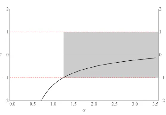
I is stable for σ<0; II, for σ >0,b >a; and V, for σ >0,a >b. (4.9) Note that I and II, as in the one-dimensional analysis of the previous section, represent the uniform homoge-neous and supercritical striped states, respectively, while V can be identified with a rhombic pattern possessing characteristic angle ϕ [10]. In the next section we shall use these criteria to refine our one-dimensional predic-tions of Figure 4(b) relevant to the former states due to the presence of the latter. Toward that end, we examine the sign of a₁±b₁. We first illustrate this procedure by defining the ratio of Landau constants [11]

(

, ; , ,

)

b1

(

, ; , ,

) (

a1 ; , ,

)

η α ϕ γ δ µ

=

α ϕ γ δ µ

α γ δ µ

(4.10)

and plotting that quantity versus

α

inFigure 5for a fixed value of

ϕ

, namely

ϕ

=0.5, and with the other parameters taking on their values ofFigure 3. Here, there exists an interval of stable rhombic patterns, where

1 1 0

a ± >b or equivalently − < <1

η

1, given by

(

1.2520, 3.5

]

[image:9.595.177.457.479.674.2]

α

∈ (4.11) provided in addition that σ >0 or β β> _c.

Figure 5.Plot of η of (4.10) for α α1< <3.5, γ =1, δ=2.5, µ =0.01,

0.5

Now, repeating the process used to produceFigure 5 but for other values of ϕ we find the same generic behavior in that there exists an interval of stable rhombic patterns for

α

∈

(

α α

m, M

]

where

1 m M 3.5

[image:10.595.171.543.317.716.2]

α <α <α = when β β> _c and summarize these results inTable 2. Then, we plot the ratio of Landau constants of (4.10) versus

ϕ

∈

[ ]

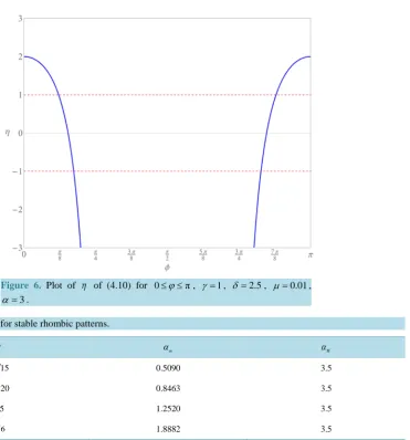
0,π in Figure 6 for α =3 and the other parameters taking on their values of

Figure 3.

Restricting ourselves to the interval of interest

ϕ

∈

[

0,π 2

]

, we see from Figure 6 that there exists a band of stable rhombic patterns for

ϕ

∈

(

ϕ ϕ

m, M

)

where 0<ϕm<ϕM <π 2 when β β> c. Observe from Figure 6

the intercept and symmetry properties

(

3, 0;1,2.5, 0.01

)

2,

(

3,π ;1, 2.5, 0.01

)

(

3, ;1, 2.5, 0.01 .

)

η

=

η

−

ϕ

=

η ϕ

(4.12)

Here, these properties of (4.12) are a consequence of mode interference occurring exactly at

ϕ

=0 and modal interchange, respectively [12]. Again, repeating the process used to produce Figure 6, but for other

1 3.5

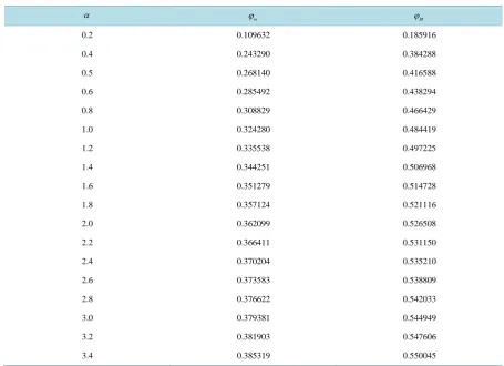
α < ≤α , we find the same generic behavior as for α =3 and summarize these results for selected values inTable 3.

Finally, we present a morphological interpretation of the stable rhombic patterns that can be associated with critical point V for the values of the characteristic angle relevant toTable 3. Then, to lowest order, the equili-brium vegetative pattern corresponding to that critical point satisfies

(

, ,

)

~ 1 A g0

( )

,z for cosz x

( )

sin

( )

,

n x y t + x =

ϕ

+y

ϕ

(4.13)

Figure 6. Plot of η of (4.10) for 0≤ ≤ϕ π, γ =1, δ=2.5, µ =0.01, 3

α= .

Table 2.Range of α for stable rhombic patterns.

ϕ α_m αM

2π 15 0.5090 3.5

3π 20 0.8463 3.5

0.5 1.2520 3.5

[image:10.595.88.539.618.714.2]

[image:11.595.84.540.96.426.2]

Table 3. Angle range for stable rhombic patterns.

α

m

ϕ ϕM

0.2 0.109632 0.185916

0.4 0.243290 0.384288

0.5 0.268140 0.416588

0.6 0.285492 0.438294

0.8 0.308829 0.466429

1.0 0.324280 0.484419

1.2 0.335538 0.497225

1.4 0.344251 0.506968

1.6 0.351279 0.514728

1.8 0.357124 0.521116

2.0 0.362099 0.526508

2.2 0.366411 0.531150

2.4 0.370204 0.535210

2.6 0.373583 0.538809

2.8 0.376622 0.542033

3.0 0.379381 0.544949

3.2 0.381903 0.547606

3.4 0.385319 0.550045

( )

, cos 2

(

πx _c

)

cos 2

(

π _c

)

.

g x y =

λ

+ z

λ

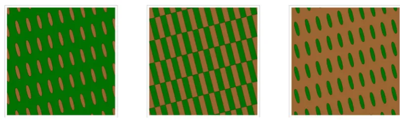
(4.14) The three parts of Figure 7are threshold contour plots of (4.14) for

ϕ

=0.5 with threshold values of 1, 0, and −1, respectively. Hence from right to left the parts of this figure can be identified with what Wollkind and Stevenson [10], Boonkorkuea et al. [13], and Cangelosi et al. [14] called upper, zero, and lower threshold pat-terns, respectively. In this context note that g x z

( )

, ≤2. Traditionally, most pattern formation analyses of this type have used the dimensional homogeneous vegetative solution value N_e of (2.4) as the threshold to trigger the color change from dark to light (seeFigure 4(a)). Thus all spatial regions characterized by N =N n_e ≥N_e appear dark and those characterized by N<N_e, light, where again dark regions correspond to high plant bio-mass density and light ones to low plant biobio-mass density or bare ground. This is equivalent to our zero threshold case of Figure 7. Note from (2.4) and (2.13) that

(

1

)

Ne

( )

k c1 .

α

=

δ

− (4.15) For fixed values of the other parameters and

δ

satisfying (2.11) we may consider

α

and N_e to be in-creasing straight line functions of R alone given by

α

( )

R and N_e

( )

R , respectively, where

( ) (

R 1

) ( ) ( )

Ne R k1c

α

=

δ

− (4.16) is a dimensionless measure of the rainfall rate R. We now wish to select a particular R=R_c and adopt the pro-tocol that

( )

c e c

[image:12.595.113.508.80.199.2]

Figure 7.Rhombic patterns relevant to g x z

( )

, of (4.13)-(4.14) for ϕ =0.5 with threshold values from right to left of 1, 0, and −1, respectively. Here, the spatial variables are being measured in units of λc and regions exceeding that threshold

in each part appear dark while those below it appear light.

Given their appearance in Figure 7we label these upper, zero, and lower threshold type rhombic vegetative ar-rays as pseudo spots, rectangles, and pseudo gaps and denote them by V+, V0, and V−, respectively, in what follows. We shall defer the specific choice for R_c, our rationale for making that selection, and its morphological interpretations until the comparison of these results with some recent vegetative pattern formation studies in-cluded in the next section.

5. Morphological Interpretations and Comparisons.

As a prelude to the morphological interpretations to be developed in this section, we first demonstrate that our model system does not generate any hexagonal patterns. We do so by considering a hexagonal-planform expan-sion for n x y t

(

, ,

)

of (2.12)-(2.13) with terms to first order given by [10]

(

)

( )

( )

( )

(

)

( )

( )

(

)

( )

1 1 2 2

3 3

~ 1 cos cos 3 2

cos 3 2

, , c c

c

A t q x t A t q x y t

A t

n y

q

x t

x y t

φ

φ

φ

 

+ _ + _+ _ − − _

 

+ _ + − _ (5.1)

where, for

(

i j k, ,

)

= even permutations of (1, 2, 3),

(

)

2

(

2 2

)

0 1 2

d

cos

4 2 ,

d ~ i j k i j k j

i

i i k

A

A

A a A A aA a A A

t σ φ φ φ



− + + − _ + + _ (5.2)

(

)

0 ~ 4 d

sin ,

d

i

i a A Aj k i j k

A t

φ _{φ φ+ +φ}

(5.3) with a similar expansion for w x y t

(

, ,

)

. Segel [15], who developed this six-disturbance methodology to analyze the Rayleigh-Bénard model of buoyancy-driven hexagonal-cellular convection, showed that the simplest way to deduce the additional Landau constants a₀ and a₂ contained in (5.2)-(5.3) was to consider its two-distur- bance reduction [16] obtained by setting

( )

( )

( )

( )

( )

( )

( )

( )

1 , 2 3 2 , 1 2 3 0,

A t = A t A t =A t =B t

φ

t =

φ

t =

φ

t ≡ (5.4) which reduces (5.1) and (5.2)-(5.3) to

(

, ,

)

1

~

(

, ,

)

( )

cos

( )

_c

( )

cos

(

_c

2 cos

)

(

3

_c

2 ,

)

n x y t

−

h

x y t

=

A t

q

x

+

B t

q

x

q y

(5.5) with a similar expansion for w x y t

(

, ,

)

where

(

)

2 2 2

0 1 2

d

d ~ ,

A

a

A a B A A

t σ − − +a B (5.6)

(

)

2 2

1 2 1 2

d

4 2 4 .

d ~ 2

B

B aAB B a a

(5.6)-(5.7) proportional to Aj

( ) ( ) (

t B tl cos Kqcx 2 cos

)

(

m 3y 2

)

with proportionality constants njlKm and jlKm

w .

Then upon substitution of (5.6)-(5.7) into (2.14) we find that (4.5) holds again while

0 0 0 0, w 0 0 0 0

jk nj K n jK jk wj K jK

n = = = =w (5.8)

for K =2k, and

0111 n1020, 0111 w1020

n = w = (5.9) as defined in Section 3. If we proceed in the same manner as we did with the rhombic-planform expansions of the last section, the Fredholm-type solvability conditions for n₀₂₂₀ and n₁₂₂₀, respectively, yield

(

)

( ) ( )

(

)

(

)

1 2

2

01 0220 01 0220

0 2 0

01 01 ; , , , 1 c c c b a a q q b β β ψ θ

α γ δ µ

µ θ ψ

= − = + − − = − (5.10)

(

)

( ) ( )

(

)

(

)

2

0 01 0220 01 1220 01 1220

2 2 2

10 01 1 2 ; , , 8 ; 1 c c c

a q b

a a

q

a b

β β

θ ψ θ

α γ δ µ

µ θ ψ

= + − + = = + − −

− (5.11)

where the components of

( ) ( ) 1 2 220 220 220 , j j j b b      =   

b (5.12) for j=0 and 1 as well as the solutions for the other relevant second-order systems are catalogued in the Ap-pendix. Observe, as pointed out by Wollkind and Stephenson [10], that the expression for a₂ of (5.11) does not contain the component ₀₂₂₀

c

n _{β β=} since its coefficient vanishes identically in this limit by virtue of (5.10), and hence is often referred to as a free mode which is why that component is not catalogued in the Appendix.

The six-disturbance hexagonal-planform amplitude phase-Equations (5.2)-(5.3) have equivalence classes of critical points given by φ φ₁= ₂ =φ₃ =0 and

I: A₁ =A₂ =A₃ =0; II: 2

1 1, 2 3 0

A =

σ

a A = A = ;

III

±: A₁= A₂ =A₃=A₀± =

{

−2a₀±_4a₀2+

(

a₁+4a₂

)

σ

_1 2

}

(

a₁+4a₂

)

; IV: A₁= −4a₀

(

2a₂−a₁

)

, A₂2 =A₃2=

(

σ σ

− ₁

) (

a₁+2a₂

)

with

(

)

2 1 0 1 2 2 1 16

2a a a a

σ

=

− .

Critical points I and II represent the uniform homogeneous and supercritical striped states described in the previous two sections;

III

± hexagonal close-packed arrays of spots and gaps, respectively; and IV, a genera- lized cell that reduces to II for σ σ= ₁ and to

III

± for

(

)

(

)

2 1 2 0

2 2 2 1 32 2 a a a a a

σ σ= = +

− [17]. Since the existence and orbital stability of these critical points depends, in part, upon the signs of various combinations of the Lan-dau constants of (5.2)-(5.3), we examine the signs of a₀, a₁+4a₂, and 2a₂−a₁ by plotting those quantities as well as a₂ versus α₁< ≤α 3.5 for

γ =

1

, δ =2.5, and

µ =

0.01

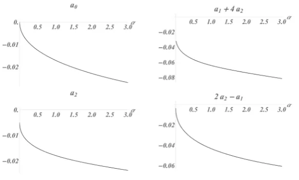
inFigure 8 and observe that they are all identically negative.

Although I is stable for σ <0, II is not stable for 2a₂− <a₁ 0 and

III

± does not exist for a₁+4a₂ <0 while IV is not stable for any set of parameter values [18]. Hence, we have demonstrated that this hexagonal- planform analysis does not yield any additional stable stationary heterogeneous vegetative patterns for our mod-el system.

Figure 8. Plots of a0, a1+4a2, and 2a2−a1 versus α α1< ≤3.5 for γ =1, δ=2.5, µ =0.01. Here, an analogous

plot of a₂ has also been included for the sake of completeness.

first summarize the simulation results of Rietkerk et al. [4]. Their two-dimensional numerical simulations of model system (1.1), with

ρ =

0

and its other parameters set at values consistent with (2.25)-(2.26), yielded close-packed vegetative patterns of spots or gaps depending upon whether R was less than or greater than 1 mm/d, respectively. Motivated by the desire to replicate this behavior and given the similarity in appearance between these two types of patterns and the right- or left-hand parts of Figure 7, respectively, as well as the fact that N_e for the Rietkerk et al. [4] model is equivalent to (2.4) of our model, we then select

1 mm d 0.5.

c c

R = ⇒α = (5.13) Thus, from our rhombic planform analysis of the previous section, we can make the prediction that V+ pat-terns will occur for R<R_c or α α< c =0.5 and V

− _{ones, for}

c

R>R or α >0.5 when β β> _c. Influ-enced by that resemblance in appearance just cited, we have referred to these periodic rhombic arrays of V± as vegetative pseudo spots or pseudo gaps, respectively. We now incorporate these two-dimensional rhombic- planform morphological stability results for

γ =

1

, δ =2.5, and

µ =

0.01

in the

α β

−

plane of Figure 9

and identify regions corresponding to the predicted vegetative patterning. Note in this context that (4.15)-(4.16), (4.17), and (5.13) imply

2

50 3 gm m .

c

N = (5.14)

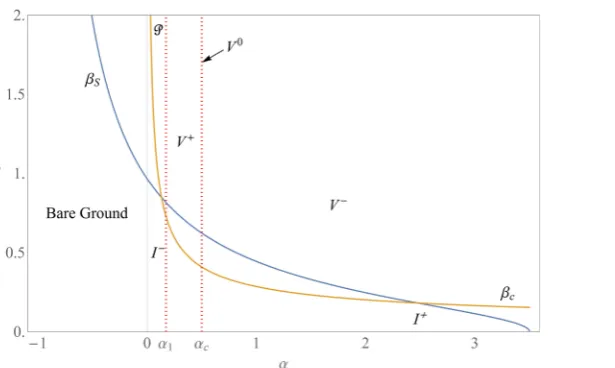
Figure 9 represents the two-dimensional refinement of our one-dimensional predictions ofFigure 4(b). Ob-serve that the occurrence of striped and rhombic patterns is mutually exclusive by virtue of stability criteria (4.9). Hence since rhombic patterns occur for all α α> ₁ in the patterned β β> _c region this precludes the occur-rence of any striped patterns there. Note that this is consistent with our hexagonal planform prediction of critical point II being identically unstable. Thus our major two-dimensional refinement of those one-dimensional pre-dictions is the replacement of the whole region of striped vegetative patterns (II) appearing inFigure 4(b) with a rhombic (V) one instead. Specifically, these are identified in Figure 9 where β β> _c as rhombic arrays of pseudo spots (V+) for α₁ < <α α_c and of pseudo gaps (V−) for α α> _c in accordance with our morphologi-cal threshold introduced in (5.13). Further, note that the 0< <β βc region of Figure 9which can be identified

with a uniform homogeneous vegetative pattern varies from a relatively sparse distribution

( 2

50 3 gm m

e c

N <N = ) for 0< <α αc to a relatively dense one (

2

50 3 gm m

e c

N >N = ) for α α> _c and hence have been designated by

I

, respectively.

[image:14.595.170.462.85.260.2]

Figure 9.Stability diagram in the α β− plane for our two-dimensional interaction-diffusion model system with γ =1, 2.5

δ= , and µ =0.01, identifying the predicted vegetative patterns. Here βS denotes the root suction characteristic of

(5.24)-(5.25) as a function of saturation with ( )0

0.22

β = .

tion equation describing vegetative pattern formation in arid isotropic environments led to the conjecture that when a₁<0 localized structures would occur where σ >0 characterized by isolated patches of vegetation at low densities that were a spatial compromise between the periodic patchy vegetation and bare ground stable states. Chen and Ward [20] found local structures occurring in conjunction with such subcriticality for the Gray- Scott reaction-diffusion chemical model system. Cangelosi et al. [14] employed the same argument to identify a region of their relevant parameter space with isolated clusters for a mussel-algae interaction-diffusion model system. The resulting morphological sequence deduced from that identification provided close agreement with mussel bed patterning observations both in the field and laboratory [21] [22]. Given the similarity of behavior among all these phenomena we conjecture with some confidence that isolated patches of vegetation would occur for 0< <α α₁ where β β> _c and identify that region graphically in Figure 9 using the designation ℘.

Taking into account the next higher-order term in the expansions and the amplitude equation of (3.1)-(3.2)- (3.3) when a₁<0 by, in particular, considering

3 5

1

1 1 1 3 1 d ~

d

A a A

A

t σ − −a A

and calculating a₃, we might enhance our understanding of the morphological stability of this system in the subcritical regime. Should a₃ >0 that equation will have three equilibrium points: Namely, 0 and

2

2

1 3 1

2Ae a 4σa a

± _{=± + − . Then 0 is stable for} 2

( )

1 a1 4a3 0

σ σ

< − = − < ;

2

e

A+ , for σ >0; and in the overlap region σ−₁< <σ 0 where both can be stable depending on initial conditions 0 is stable for

( )

2

2 1

0<A 0 <A_e− and A_e+2, for 2

( )

2

1 0 e

A >A− , while A_e−2 only exists in that bistability region but is not stable there [23]. Here the potentially stable equilibrium points 0 and Ae2

+

would correspond to

I

− and ℘, respectively.

Determining the generalized marginal curve for our problem analogous to (2.24) but with σ ≠0 we would find that [see Kealy and Wollkind [24] for the derivation procedure involved]

(

)

1 2

(

)

₂ 1 2

(

)

; , , 2 1 ,

σ

µγ

µ σ

µ

β α γ

µ

α

γ

α σ σ

µ

α

α

∆ ∆ + + ∆ + +

∆

+

= _

∆

  +



where

β

σ=₀

(

α γ

; , ,∆

µ

)

=

β α γ

c

(

; , ,∆

µ

)

. Plotting the marginal curve associated with σ σ= −1,

(

)

₁

(

)

(

)

1 ; , , σ ; , , c ; , , ,

β β α γ

µ

β

α γ

µ

β α γ

µ

−

− ∆ = ∆ < ∆

=

[image:15.595.182.490.82.266.2]

appearing in this figure only due to the presence of the overlap region β₋₁< <β β_c where ℘ as well as

I

−

patterns could now occur. Should a12

( )

4a3 1, as was the case for a similar situation in Kealy and Wollkind

[24] involving hexagonal patterns, the marginal curves would coincide or β₋₁ ≅β_c causing the overlap region virtually to disappear and resulting in the exact same identifications as the ones appearing in Figure 9.

Traditionally, morphological sequences of the sort referred to above have been generated from stability dia-grams such as Figure 9 by traversing appropriate horizontal or vertical lines in that two-component parameter space (e.g., Cangelosi et al. [14]; Kealy and Wollkind [24]). A procedure of this sort is inherently dependent upon the implicit assumption that these two components are independent of each other. In the case of Figure 9, however,

α

and

β

, being nondimensional measures of rainfall and the coefficient of plant root suction, re-spectively, are actually related. To obtain the proper morphological sequence of vegetative states along a rainfall gradient predicted from Figure 9, it is first necessary for us to deduce that relationship. Toward this end, em-ploying our basic definitions and the parameter values of (2.25)-(2.26), we find that

(

4

)

gm d mm m .

S W S

c cD D D

β = ρ= = ⋅ ⋅ (5.15) Note in (5.15) the units for D_S as indicated below, are mm m4/(gm⋅d) consistent with

β

being a dimen-sionless parameter. Adopting the root suction characteristic of Roose and Fowler [25], we take

( )0

_{( )}

4

₍

₎

mm m gm d

S m

D =β f S ⋅ ⋅ (5.16) where

( )

(

₁

)

1

1 m for 0 1 and 0 1.

m m

f S = S− − − < <m < ≤S (5.17) Here S≡ the relative water saturation in the soil while the parameters

β

( )0 and m are determined from experimental data for different soils. To complete our formulation we let

for 0 mm d

M RM

S=R R < ≤R (5.18) where, specifically,

3 mm d .

M

R = (5.19) Upon recalling that

(

) (

)

1 1

R=k d

α γ

+

δ

− (5.20) and substituting (5.20) into (5.18)-(5.19), yields

(

) (

M

)

for 0 M

S=

α γ

+

α

+

γ

α

< ≤

α α

(5.21) where, specifically,

0 1, M 3.5.

α = − = −γ α = (5.22) Hence

(

1 4.

)

5 for 1 3.5.

S=

α

+ − < ≤

α

(5.23) Finally, selecting m=0.5 after Roose and Fowler [25], and incorporating (5.23) and (5.16)-(5.17) into (5.15), we obtain the one-parameter family of root suction characteristic curves

( )

( )0 0.5

4. 1

for 1 3 5

5 .

S f

α

β β α =β _ _ α

  − < ≤

+

= (5.24)

where

( )

(

)

1 2 2

0.5 1 .

( )

0,2

( )

0,2

S p c p

β =β (5.26) where, specifically,

0 0.13217, 2 2.47622.

p = p = (5.27) Here, from (5.20), these

α

-values of (5.27) correspond to

0 0.75478 mm d , 2 2.31748 mm d ,

R = R = (5.28)

respectively. In this context, we define

1 c, 1 0.78133 mm d

p =α R = (5.29) where

α

( )

R1 =

α

1. The morphological sequence of predicted stable vegetative states along a rainfall gradient

obtained upon traversing the curve

β β α

= _S

( )

in the

α β

− plane ofFigure 9 is tabulated below. Note, in general, that

( )

0 1

0

if 0.20.

p α β

< >

   

 ₌  ₌

   

 _>  _{ <} =



(5.30)

Thus, isolated patches are only predicted for transit curves of the form of (5.24)-(5.25) provided

β

( )0 >0.20. We next compare these theoretical predictions with relevant observational evidence. The relevant reported vegetative patterns [2] consist of spots (leopard bush) and gaps (pearled or spotted bush). After Boonkorkuea et al. [1], we now associate our rhombic arrays of pseudo spots (V+) or pseudo gaps (V−) with these leopard or pearled bush vegetative patterns, respectively, and then investigate the predicted wavelength of those vegetative patterns. From (2.24) and (3.8), we can deduce that

( )

4 4

2π .

c c

λ

=

µ

∆

α λ α

= (5.31)

Designating the

α

’s associated with V± by α±, respectively, it follows fromTable 4 that

1 2

1 c p p .

α

_{< <}

α

+_<

α

_{= <}

α

−_<

(5.32) Then, we can see from (5.31) and (5.32) that

( )

( )

,

c c c

λ+ ₌λ α+ _>λ− ₌λ α− _(5.33) and hence conclude that the vegetative distributions of spots in leopard bush have a tendency to be more widely spaced than the bare patches which regularly punctuate the vegetation cover in pearled bush [26]. Employing the length scale of (3.8) and the parameter values of (2.25)-(2.26), yields the associated dimensional wavelength re-lationships

m 19 m 12.7 m

25 >

λ

_c∗+> >

λ

_c∗− > (5.34) consistent with field observations and in agreement with Boonkorkuea et al. [13], who interestingly enough found an identical power law relationship to (5.31) between their pattern wavelength and plant biomass for the evolution equation of Lejeune et al. [19].

transi-tion between the two hexagonal states occurring exactly where the second-order Landau constant changed sign [13]. Gowda et al. [27] concluded that weakly nonlinear stability theory failed to produce the correct results in the first instance because the simulated morphological sequence of vegetative patterns occurred for large ampli-tudes as the precipitation parameter was decreased. Given our results, we wish to suggest another possible ex-planation for this discrepancy: Namely, that a rhombic-planform weakly nonlinear stability analysis might yield a predicted morphological sequence involving pseudo gaps → rectangles → pseudo spots as the precipitation parameter was decreased in this case. As supporting evidence for such a conjecture we offer the following ob-servation. The gap- and spot-type simulated patterns for 1µ =100 appearing in both Gowda et al. [27] and von Hardenberg et al.[1] were much less regular in nature than were the corresponding simulated hexagonal patterns for 1µ =27 appearing in Gowda et al. [27]. The simulated transition states between these two types of patterns were also different consisting of labyrinths in the former instance but of parallel stripes in the latter case. Since for each value of α we predict multistable rhombic states with an interval of characteristic angles (see Figure 6 andTable 3) and as initial conditions vary point by point over a flat environment these states can be selected quite randomly, it is possible to generate simulated patterns resembling those appearing in von Har-denberg et al. [1] from families of pseudo gaps and pseudo spots including labyrinths from families of rectan-gles. Incidentally these labyrinthine patterns have been associated with certain types of so-called tiger bush or banded thicket vegetative distributions found in arid or semiarid flat environments [28]. In this context, the nu-merically simulated two-dimensional patterns of Rietkerk et al. [4] used earlier to motivate our choice for R_c also bore a strong resemblance to those of von Hardenberg et al.[1] including a labyrinthine transition state at

m d 1 m

R= . Unlike the von Hardenberg et al. [1] model ours is extremely robust to variations in µ. We per-formed additional rhombic and hexagonal planform nonlinear stability analyses on system (2.14) and found identical qualitative behavior for all 0.001≤ ≤

µ

1.

We end this phase of our discussion by restating von Hardenberg et al.’s [1] claim that the power of model systems such as ours of (1.5) is their predicted sequence of stable states along a rainfall gradient such as the one summarized in Table 4 can be used to motivate an aridity classification scheme which is characterized by the three rainfall thresholds

0 0.13217 p1 0.5 p2 2.47622.

p = < = < = (5.35) Here we are employing the notation of von Hardenberg et al. [1] for these dimensionless rainfall (precipita-tion) rate thresholds and use them to introduce the following possible aridity classes based upon the inherent vegetative states of our system:

• Dry-subhumid (p₂< <α 3.5): The only vegetative state the system supports corresponds to a dense homo-geneous distribution.

• Semiarid (p₁< <α p₂): The only vegetative state the system supports corresponds to pseudo gaps of low threshold type.

• Arid (p₀ < <α p₁): The only vegetative states the system supports correspond to either pseudo spots of high threshold type or isolated patches.

[image:18.595.87.536.574.721.2]

• Hyperarid (− < <1 α p₀): The only possible stable states the system supports correspond to either a sparse homogeneous vegetative distribution or bare ground.

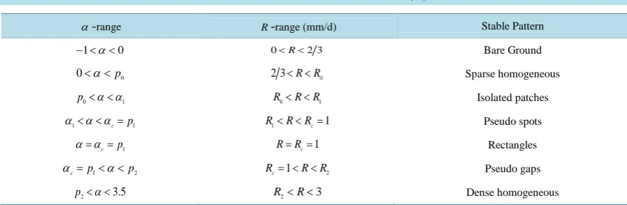
Table 4.Morphological stability predictions along a rainfall gradient for β β α= _S

( )

in Figure 9.

α-range R-range (mm/d) Stable Pattern

0

1 α

− < < 0<R<2 3 Bare Ground

0

0< <α p 2 3< <R R0 Sparse homogeneous

0 1

p < <α α R0< <R R1 Isolated patches

1 c p1

α α α< < = R1< <R Rc=1 Pseudo spots

1

c p

α α= = R=Rc=1 Rectangles

1 2

c p p

α = < <α Rc= < <1 R R2 Pseudo gaps

2 3.5

As pointed out by von Hardenberg et al.[1] the advantage of the proposed aridity classification scheme per-tains to the information it conper-tains about dynamical aspects of drylands. Regions whose aridity classes imply the occurrence of upper threshold vegetative patterns, isolated patches, or a sparse homogeneous distribution are vulnerable to desertification. The mere knowledge of that threat, however, allows land managers to reverse this process for those regions by implementing crust disturbance, seed augmentation, or irrigation strategies. Meron et al. [29] suggested a cycling mechanism between plants and water to account for the formation of bare patches characteristic of vegetative patterning along such a precipitation gradient. Note that a process of this sort occurs in all directions for two-dimensional vegetative patterns (pseudo spots or gaps, rectangles, and isolated patches) but only in two directions for one-dimensional ones (stripes).

We close with a more detailed commentary on the role played by cross-diffusion in generating pattern forma-tion instabilities for our two-component model system. Given that θ =₁₀ 0, our system violates the activator positive feedback necessary condition for the occurrence of a Turing self-diffusive instability which requires

10 0

θ > . Hence the cross-diffusive effect of plant root suction on ground water generates our instability since as noted earlier if

β

=0 its community equilibrium point would be identically linearly stable. Indeed, the other requirement of

µ

<1 for a Turing self-diffusive instability to occur might also be violated should

µ

=1, and a cross-diffusive instability of this type could still be generated although, in our actual parameter range, it is not violated. Recently, Stancevic et al. [30] considered a reaction-chemotaxis-diffusion three-component in-host viral dynamics model system for the concentrations of uninfected or infected cells and the virus. They found that the cross-diffusive effect of chemotaxis toward the infected cells by the uninfected ones generated their pattern formation instability in a similar manner as for our two-component system. Since the community equilibrium point of their system was linearly stable in the absence of diffusion and chemotaxis, Stancevic et al. [30] re-ferred to this as a Turing instability. To distinguish between these two cases, we shall refer to ours as a Turing cross-diffusive instability instead. The von Hardenberg et al.[1] two-component nondimensional model system also included the cross-diffusive effect of plant root suction on ground water. Since that system’s interaction terms satisfied the activator positive feedback condition for its community equilibrium point while 1µ =100 in their default set of parameter values, the presence of this cross-diffusive effect mediated rather than generated their Turing self-diffusive instability. In particular, von Hardenberg et al. [1] took the coefficient of that term

3

b= in this default set. Upon inspection of (2.14) we can see that this coefficient is related to our parameters by

.

b=αβ (5.36) Thus that assignment would yield the root suction characteristic curve

3 ,

β= α (5.37) which, as a decreasing function of

α

is in qualitative accord with our formulation of (5.24). The three-compo- nent model systems of Rietkerk et al. [4] and HilleRisLambers et al.[5] by explicitly including surface water were able to generate Turing instabilities where none would have occurred for our simplified two-component version of that model without root suction. Finally, Wang et al.[31] conducted a definitive analysis of Turing instabilities for their predator-prey model system by including both self- and cross-diffusion terms in the prey and predator equations and performing weakly nonlinear hexagonal-planform bifurcations and numerical simu-lations on its community equilibrium point. Since the Allee positive feedback effect for the activator prey and the self-diffusivity advantage for the inhibitory predator were satisfied for their specific model, this was an in-vestigation of cross-diffusion mediated rather than generated instabilities.

6. Conclusions