A game theoretic approach to pollution control problems

Munich Personal RePEc Archive

A game-theoretic approach to pollution

control problems

Halkos, George

University of Thessaly

1994

Α game-theoretic approach to pollution control problems

Βy

George Ε. Halkos

ABSTRACT

This paper provides a model that attempts to deal with the transboundary nature of the acid rain problem, using a game theoretic approach consistent with mainstream economic theory. The general forms of cooperative and non-cooperative equilibria in the explicit and implicit set-up of the model are presented under the assumptions of deterministic and stochastic deposits.

JEL classification codes: Q2, C7

Keywords: Game theory; abatement cost; damage cost.

____________________________

An earlier version of this paper has been presented as:

Halkos, G., 1994. ‘A game-theoretic approach to pollution control problems’, Department of Environmental Economics and Environmental Management, Discussion Paper Series, Number

Introduction

Much has been written recently about the use of negotiation and bargaining to resolve

environmental conflicts. Negotiation and bargaining occur between governments to attempt to

settle conflicts concerning land use, energy and air quality (Bingham, 1986). Bargaining has

generated much theoretical interest, beginning with the classic work of Nash (1950, 1953) and

Raiffa (1953). Until a few years ago, most theoretical work assumed complete information, i.e.

the bargainers' utility functions, the set of feasible agreements and the recourse options

available if bargaining failed were all considered to be common knowledge. According to this

assumption, the problem was explored using one of the following approaches:

i) The first approach was presented in Nash (1950, 1953) and Raiffa (1953) and was extended

and completed recently by Roth (1979), has not tried to describe the bargaining process

explicitly through a specific extensive form. Rather, it has concentrated on formulating and

exploring the implications of general principles that are compatible with possibly many

different extensive forms. This approach is often described as "cooperative" since the

jointly agreed-upon solution is implemented presumably by a binding agreement (Roth,

1979).

ii) The second way of exploring the bargaining process specifies a bargaining game, whose

equilibrium outcome then serves as a predictor of the outcome of the actual bargaining

process. The Nash solution is only one of many equilibria of a simple one stage demand

game in which players make demands simultaneously and the agreement occurs if the two

demands can be met by a feasible agreement. If the demands are not compatible in this

way, a conflict occurs and two possible disagreement outcomes can be considered:

- the status quo which corresponds το zero welfare improvements for each

- the non-cooperative Nash equilibrium i.e. the equilibrium point without any

pre-play activity between the bargainers (Harrison and Rutstrom, 1991; Binmore

and Dasgupta, 1990; Roth, 1979).

The latter, as will be seen, is the “conflict point” in the model proposed here. In fact, it will be

seen that such a model is fully consistent with the approach outlined above as point (ii).

Each of these approaches has its strengths and weaknesses. Specifying an extensive

form enables us to model the strategic use of private information and, therefore, has

implications that could be proved useful for individual bargainers. However, an extensive form

is bound tο be arbitrary to some extent and the axiomatic approach cuts through disputes about

choice of extensive forms (Roth, 1979).

On the other hand there are models of bargaining which assume incomplete

information. These models are concerned with situations where each party has private

information (e.g. about preferences) that is unavailable to the other parties. This relaxation of

the assumptions made in the complete information framework has crucial implications. The

most interesting one for economists is the persistence of Pareto-inefficient outcomes in

equilibrium, the most striking of which is the existence οf disagreement even when mutually

beneficial agreements exist. As before in the case of complete information models, the

theoretical studies with incomplete information have employed two somewhat different

research strategies. The axiomatic approach was pioneered by Harsanyi and Selten (1972). The

strategic approach is based οn Harsanyi (1967, 1968), whose work supplied the extension of

the Nash-equilibrium concept essential tο explain games of incomplete information.

ln this paper it is first assumed that before strategies are chosen in a formal game played

cooperatively, players have complete information, i.e. they may communicate costlessly and

without restrictions, and they may choose to enter into any agreement. The non-cooperative

from it (Basar and Olsder, 1982; Mehlmann, 1988; Kaitala et al., 1992). Here two types of

equilibria are considered. One is the "social welfare" agreement that seeks to achieve

maximum aggregate net benefits. The benchmark against which to judge the benefits of

cooperation is, of course, the status quo, which we take to be the "naive" non-cooperative Nash

equilibrium. Net benefits in the former case of equilibrium may be distributed unevenly and

even be negative for some countries (Mäler, 1989, 1990; Halkos, 1994). Ιn this case, we

identify the need for "side-payments" to induce agreement: clearly such side-payments need

not be financial, but could be in the form of compensating net benefits from agreement on

other issues.

Papers by Hoel (1991), Shogren and Crocker (1991), Mäler (1989, 1990), Harrison and

Rutstrom (1991), Kaitala et a1. (1992) and Tahvonen et al. (1993) explore the economics of

cooperative and non-cooperative solutions in pollution control problems. Mäler provides a

clear analysis of the "acid rain game" and some estimates of the gains from cooperation for

European countries; Kaitala et al. (1992) and Tahvonen et al. (1993) model a dynamic game

between Finland and four regions of the former USSR. Hoel considers a global pollution

problem where all players are affected by the same amount of pollution. Relying on standard

economic theory he reinterprets the classic welfare economic theory into a game theoretical

framework's without any empirical implementation. In general, it can be said that all these

studies provide general forms of cooperative and non-cooperative equilibria but none of them

gives any example of an explicit solution.

The idea presented in this paper is that, instead of seeking the cooperative equilibrium

values of abatement and then re-distributing the resulting total abatement cost across countries

according to some more "equitable" criteria, one could directly seek the Nash and cooperative

equilibria. This would incorporate at least some of the "equitability" requirements since the

pollution control. Moreover, the difference between the Nash equilibria and the cooperative

ones could be used as the basis for evaluating each country's gain (or loss) from the coalition.

Ιn this case the "equitability" of the cooperative equilibrium could as well be put into

discussion. This is because the benefits from cooperation are stated in "efficiency" terms: a

cooperative policy bargain can be made which leaves some countries better off, without any

other ones being left worse off, i.e. a Pareto preferred bargain.

This paper considers the implications of relaxing the assumption of complete

information. It is organized as follows. Sections 1 and 2 introduce formally a simple model in

implicit forms under the assumptions of perfect and imperfect information. Similarly, section 3

presents the formulation of the model in explicit terms. Section 4 provides an empirical

application of such a model. Finally, section 5 presents some concluding remarks.

1. Α PROPOSAL FOR MODELLING EMISSION CONTROL STRATEGIES

In this section the behaviour of countries adopting emission-control strategies is

investigated in the following simple model. Let us suppose that Ν countries, labelled i=

1,2,...,Ν produce a single good, electricity, denoted Yi, through the use of fossil fuels. Along

with electricity, a "bad" output, sulphur emissions, denoted Εi, is also produced, through the

combustion of fossil fuels. The Ν countries are assumed tο be a subset of the total number of

countries in the world and the amount of emissions caused by each country is a function of the

electricity they plan to produce, i.e.:

Ei=Ei(Yi) i = 1, 2, ... , Ν (1)

The transboundary nature of the acid rain problem is represented by the following

expression Di = Bi + dii (1- αi)Ei + Σij dij (1- αj)Ej (2)

where Ei and Ej are the total sulphur emissions per unit of time in country i and j respectively;

country i; dij are sulphur depositions in country i per unit of sulphur emissions in country j, i.e.

the transfer coefficient from country j to i. Similarly, dii are sulphur depositions in country i per

unit of sulphur emissions in country i. The proportions of emissions from any source country

that are ultimately deposited (in the form of acid rain) in any receiving country are presented in

the European Monitoring and Evaluation Program of the Norwegian Meteorological Institute

(see ΕΜΕΡ, 1993)(1)_{. B}

i is the level of background deposition attributable to natural sources

(such as volcanoes, forest fires, biological decay, etc) in receptor-country i, or to pollution

remaining too long in the atmosphere to be tracked by the model, i.e. is probably attributable

not only to natural sources but also to emissions whose origin cannot be determined (2)_{. Then}

equation (2) reduces to

Di = Bi + Σj dij (1- αj)Ej (3)

Sulphur deposits cause physical damage which can be measured and expressed in

monetary terms, using the damage function

Qi = Qi(Di) i= 1,2, ... ,N (4)

which is assumed to be strictly convex in Di, i.e. Qi'(Di) >0 and Qi"(Di) >0. For the damage

functions, the existing literature assumes that damage is a linear function of depositions (see

Mäler, 1989, 1990; Newbery, 1990). The evidence of sensitivity maps, however, strongly

indicates that this is not valid, and that the damage function should be convex: doubling the

rate of deposition will more than double the damage caused. Halkos (1992) and Halkos and

Hutton (1993) have shown that assuming a linear damage cost function gives the Nash as a

dominant market equilibrium. It is also notable that if the true damage cost function is convex

instead of linear, which seems probable (and it is assumed in this paper later on) then this will

yield an overestimate of the gains from cooperation, as the marginal benefits from reductions

in sulphur deposits will be overstated. Also, quadratic damage functions yield interdependence

we will infer its parameters by assuming that countries currently equate national marginal

damage cost with national marginal abatement cost.

Given the above, let us suppose that countries face three types of costs:

- first, production costs, denoted PCi, which will be considered as a datum in the

model;

- second, costs of abatement, denoted CΑi(Εi,α), where αi is, as mentioned,

country i's abatement coefficient; and

- third, damage costs, denoted, as in expression (4) above, Qi=Qi(Di).

In discussing costs of abatement, we need to distinguish between primary and secondary

abatement. Primary abatement can be done by fuel switching to low- or sulphur-free fuels, by

reducing the use of sulphurous fuels as a result of improved fuel efficiency in power plants,

and in general by any other measure reducing the output of electricity. Secondary abatement

cost functions measure the cost of eliminating tonnes οf emissions before (e.g. coal washing),

during (e.g. by Fluidized Βed Combustion), or after (e.g. Flue Gas Desulphurization) burning

the fuel(3)_{. These vary between countries depending on specific characteristics like fuels used,}

sulphur content of these fuels, existing or new power plants and on the local costs of

implementing best practice abatement techniques. Full details οn the secondary abatement

cost functions used here are reported in Halkos (1992, 1993, 1994).

In the model proposed in the next section, we assume quadratic (convex) abatement

costs, as do Kaitala et al. (1992) and Mäler (1989, 1990). Our purpose is to rely on the level of

existing secondary abatement in each European country (if any) and in this way, to assess the

optimal contribution of secondary abatement in reaching the environmental targets imposed by

current agreements ("30% Club", "New Sulphur Protocol") and to expose the role of primary

abatement(4)_{. Let us now consider, in turn, the non-cooperative and cooperative equilibria}

2. IMPLICIT FORMULATION OF THE MODEL

2.1 Assuming complete information

The Nash equilibrium concept is based on the assumption that countries do not

negotiate or communicate in any other way regarding their environmental policies; each

country acts in a non-cooperative way taking the environmental policy of other countries as

given. It is assumed that countries are rational and behave like Cournot (Nash) duopolists, in a

non-cooperative game theoretic framework. Then the net benefit from electricity production of

each country, denoted ΝΒi(Υi,αi) will be defined as the difference between the value of

production, pi Yi, where pi=pi(Yi) is the market price of electricity in country i, and the above

mentioned three types of costs, i.e.:

ΝΒi(Υi, αi) = pi (Yi)Yi – PCi – CAi(Ei,αi) –Qi(Di) (5)

Considering this simple model from a game theoretic point of view, it can immediately

be seen that the Nash equilibrium is ensured by those values (αi*, Yi*) which solve the

following problem:

maximize NBi = pi Yi – PCi – CAi(Yi,αi) –Qi(Yi, ΣjYj, αi, Σjαj) (6)

subject to pi = pi (Υi)

for country i. Another theoretical possible non-cooperative equilibrium is the Von Stackelberg

solution according to which one country is assumed to have superior information (for more

details see Halkos, 1992; Halkos and Hutton, Ι994).

However, the transboundary nature of the acid rain problem makes it obvious that some

kind of cooperation between countries could be needed. More specifical1y, one must consider

the terms of bargaining between countries embodied in the model, where the term bargaining

means the negotiations between countries about the terms of possible cooperation in pollution

control. One possible way of defining a cooperative equilibrium abatement strategy could be

Maximize Σi NBi

αi, Yi

subject to 0 αi 1 (7)

The solution concept to this problem implicitly requires transferable utility, i.e. that gains in

one country can be transferred to other countries in order to achieve another distribution of

gains and losses.

2.2 Assuming imperfect information

Under complete information, all players by assumption know the exact payoffs

(benefits) that their opponents can obtain. This is a demanding assumption. Το assign the

benefits from certain actions it is necessary to know the expected benefits each player obtains.

But expected benefits capture individual characteristics such as attitudes towards risk. In this

section the analysis will be carried out with the assumptions of incomplete information and risk

neutral players.

For our purposes, it can be said that acidic emissions may be deterministic in the sense

that countries are able to choose adequate abatement strategies to determine the final level.

Conversely, deposits of each country could be considered as a continuous random variable due

to the influence of atmospheric and geologic factors that countries cannot really control and

some probability limits can be assumed. We could think of a probability density function fi(Di)

of the actual level of deposits Di in i=1,2, ... ,Ν different countries to be defined in an interνal

[Bi, Βi+Πi) such that

( ) ( ) 1

i i i

B

i i i B

f D d D







where Βi denotes background deposits explained above and Πi for ij is defined as:

1

1 N

i ij j ii i j

d E d E





Therefore, the possibility for countries to set adequate abatement efficiency influences

only the range in which the final value of the (continuous and strictly positive) random variable

Di is more likely to occur. Α greater probability of occurrence for values nearer Bi+Πi is due to

the fact that high levels of deposits certainly cause a negative externality to the country, but

abatement cost increases more than proportionately with the amount of pollutant removed so

that lower levels of (αi, Σjαj), would determine energy cost savings for the countries, although

at the "price" of higher deposits. It is worth mentioning that it is not only weather that

determines the range of Di for a given pattern of emissions. As we have seen, the energy cost

savings made possible by higher deposits, i.e. lower abatement levels, cause an asymmetric

behaviour of the probability distribution of deposits and therefore a greater occurrence of

values of Di nearer to Βi + Πi.

Therefore, both equation (9) and the argument that deposits are depletable (i.e. what is

not deposited in one country must be necessarily distributed among the others, or some others),

allow us to consider deposits in different countries as dependent random variables, whose joint

probability density function is defined as follows:

( , )i j i( ) ( / )i j j i

g D D  f D f D D (10)

Of course, g(Di, Dj) would be such that:

( , ) ( ) ( )

j j j

B

i j j i i

B

g D D d D f D







according to the statistical definition of marginal distribution.

Recalling that emissions do not only cause damages of various kinds but also produce

"benefits" such as the mentioned energy cost savings (made possible, for instance, by the use

of high rather than low sulphur content fuels, so that resources otherwise allocated to

abatement with the emission reductions, country’s i expected benefit from pollution control can

1 ( , ) ( )

j j i i j i j

B B

N

i j i j i i j i i

j B D D

EB c g D D D dD dD CA D

 

 _



  

where cj is the marginal abatement cost per unit of pollutant removed and CAi(Di) is the

abatement cost. Expression (12) represents, for each of the i= 1, 2, ..., Ν countries, the so-called

"payoff function": the double-integral's setting and limits appear then more clear, in so far as

they show that countries quantify their uncertainties -in this case, concerning deposits - using

subjective probability distributions and taking the other countries' behaviour as given (see the

second integral's lower limit Di=Dj in expression (12). Similarly, expression (10) defines for

each of the i=1,2,...,N countries the so-called "beliefs", represented in game theory by

subjective probability distributions over a set of possible "states of the world" -described, in

our case, by the occurrence of different deposition levels.

In turn, the introduction of an explicit deposits target Di to be met by the country under

consideration (for instance, a single country might want to pursue its own deposition target

independently of any joint action with other countries) would modify expression (12) as

follows:

1 ( , ) ( , ) ( )

j j i i i

j i j i i

B B D

N

i j i j i i j i j i i j i i

j _{B D D B}

EB c g D D D dD dD g D D D dD dD CA D

   _{ }           

  



where the term i i i ( , )

j i i

B D

i j i i j B B

g D D D dD dD







 

3. EXPLICIT FORMULATION OF THE MODEL

3.1 Assuming complete information

Some specific functiona1 forms for total damage and abatement costs can now be

assumed, for the purpose of giving an example of "efficient" emission control policy, which

will show how each country's abatement strategy is able tο influence the strategies of other

countries in a non-cooperative game theoretic framework such as the one sketched so far. For

instance, assuming quadratic total damage and abatement costs in deposits and emissions

respectively, i.e. TCdamage,i=γi Di2, where Di is given by expression (3) and ΤCabatement,i=βi(αiΕi)2,

where αi indicates country i's abatement coefficient, Εi its unconstrained emissions and γi and βi

are parameters explained later on (in section 4), then the total cost that country i will seek to

minimize is

Ci=TCproduction, i+ TCabatement, i + TCdamage, i = TCproduction, i+ βi (αi Εi)2 + γi Di2 (14)

The first order conditions (FOCs) Ci/ i 0will give us the reaction function of each

country i and the solution of these Ν FOCs will give us the Nash non-cooperative equilibrium

values. It is implicitly assumed that the abatement values lie between 0 and 1 (i.e. 0αi1)

because they are obtained from an "unconstrained" minimization problem (simply

(Ci/ i 0).

Similarly, the cooperative set-up of the model can be written as follows:

Minimize Σi Ci

αi

(15)

subject to 0  αi  1

The combination of abatement which minimizes the total abatement costs and social

environmental damage costs across countries will be referred to, in this case, as the social

and these conditions will give us first the reaction line of each country i, and then the unique

cooperative or "social-welfare" equilibrium values.

3.2 Assuming incomplete information

Let us consider Di as a continuous random variable and let us assume a certain

probability value comprised between "reasonable" limits, that is, within a finite support which

will be formed by an "upper bound" deposition level, called DUi, and a lower bound level,

called DLi. Such bounds will be defined as:

(1 )

Li ii i i i

D d     αj=1 (16)

(1 )

Ui ii i i j ij j i

D d     d    αj=0 (17)

In other words, (16) assumes that countries are actually practising the maximum abatement, as

it can be obtained by setting αj=1 in expression (3); whereas (17) assumes that countries are not

abating anything, so that country i receives the entire proportion of all other countries'

emissions ΣjdijEj as proved by setting αj=0 in (3).

Then, in order to keep the analysis simple it will be assumed that deposits are equally

likely tο assume values between the lower and upper bounds defined so far; i.e. we assume that

deposits are determined on the basis of a uniform probability function, which will be defined as

follows:

1 ( )

i i

Ui Li

f D

D D



 i=1, 2,…, N (18)

Having then introduced this "new" definition of deposits, we can examine, again in the

case of country i for our expository purposes, what the total costs for that country become. In

fact, using (18), the minimization of the sum of production, abatement and random damage

Minimize (19)

That is the difference between (19) and, for instance, (14) in the case of certainty, is

represented by the random term in damage costs, given by expression (18), which clearly

models country i's “expectations” concerning the value of its own deposits, and therefore of its

own damage cost. Notice that in this way (i.e. by allowing for random deposits) the somewhat

restrictive assumption of country i having complete information about countries j' s abatement

coefficient values αj -necessary for deriving the Nash equilibrium set-up of the model under

certainty- is avoided here.

In this more reasonable case, country i does not have perfect information concerning

countries j's abatement strategies but, as we wil1 see, a Nash equilibrium will still be possible,

since country i, by expression (18) is able to compute a subjective probability over the other

countries' behaviour and therefore over its own costs which must be minimized. Returning to

expression (19) and omitting, for reasons of simplicity, the cost of production, we obtain:

Minimize (20)

so that, as already mentioned, the Nash equilibrium abatement rates can be found by solving

the FOCs, TCi/ i 0, which will give us first the reaction functions of each country i and

then the Nash solutions.

Comparing the FOCs of problems (20) and (14) it can be said that country i's abatement

coefficient under the assumption of "stochastic" deposits will be smaller than the abatement

coefficient that country i would select under the assumption of "deterministic" deposits only if

( 0.5) 0 j ijd Ej j

   (21)

We can then conclude this part of the discussion by saying that market equilibrium may

such equilibrium presents some "inefficiency" with respect to the certainty Nash equilibrium,

since it leads to abatement choices that might overestimate - or underestimate -the real damage

they will cause. However, the question whether something "better" could be attained by some

kind of joint action or cooperation with other countries is quite significant in the analysis of the

economics of acidification in Europe.

Let us now consider the cooperative set-up in the case of incomplete information.

Recalling (20) we have:

Minimize

(22)

and solving the FOCs (i.e. SW/ i 0) we can derive the abatement coefficients under

uncertainty for each country i. Then, comparing the FOCs of problems (22) and (15), it can be

said that if

2

2 2 ₁ 2

3

j j ii i i ii j j ii i ii

d

d d d 

       

or 2 2 1

3

j j ii i

d



   

then country i's abatement coefficient under uncertainty will be smaller than the abatement

coefficient that country i will choose under certainty. This makes sense because countries

under certainty are prepared to abate more than under uncertainty.

Finally, cooperative and non-cooperative solutions of the game embodied in the

proposed model could be compared to assess the benefits of cooperation. The empirical

evidence οn the magnitude of these potential cooperation gains suggests that they might be

quite significant (Mäler 1989, 1990; Halkos, 1994). In this respect, the social welfare

maximizing case becomes fully relevant. The model presented in this section could then be

regarded as a useful "tool" to describe and interpret such a reality: for this reason, in the next

4. ΑΝ EMPIRICAL APPLICATION OF THE MODEL

4.1Simulation

Preliminary steps need to be considered, which relate to the fact that it is the monetary

values of abatement and damage costs that must be considered in the empirical test of the

model. More precisely, the total-cost formula was:

TCi = TCabatement, i + TCdamage. i =ii2Ei2 + γi Di2

where TCi the total cost of country i (i=1,2,...,Ν). The method used to estimate the monetary

coefficient βi is the following. First, the relationship

TCabatement, ik = a +bi TSRik2 + uik

for country i and for the value k of TSR (= αiEi), is estimated by ordinary least squares (OLS);

and where a is a constant, u is a disturbance term and TSR is the tota1 amount of sulphur

removed(5)_.

We calibrate the damage function by assuming that nationa1 authorities act as Nash

partners in a non-cooperative game with the rest of the world, taking deposits originating in the

rest of the world as given. Το obtain the damage cost's monetary value γi we have:

TCi = [a +bi (αi2 Ei2)] + γi [dij (1- αi)Ei + Σij dij (1- αj)Ej]2

Then, letting the first derivative of the above with respect to αi be equal to zero gives:

2

0 2 2 ( ) 0

i

i i i i i ii i i

TC _{b E  D d E}





   



i.e. i( i i)

i

ii i

b E

d D



 

In order to model the politica1 unification of Germany, the damage coefficient of the FRG has

been used for both countries (FRG and GDR) for the year 2000. The trade-off of sulphur on

which the results of the paper are based is drawn from the ΕΜΕΡ model. This is based on the

old European boundaries. However, it turns out that it is useful to work with "old data". It does

boundaries because historic policies in the two areas have been so different. Also, as our

calibration is based on the year 1990 it is necessary to treat the former USSR and

Czechoslovakia as political units even in the year 2000.

Finally, the unconstrained sulphur emissions used here are based on research conducted

by IIASA for the years 1990 and 2000. The emissions for the year 1990 are net (i.e. after

secondary abatement) while these for the year 2000 are gross (Amann and Sorensen, 1991).

For 1990 and for calibration of the damage function, we have estimated gross emissions using

the existing secondary abatement level of European countries in 1990.

4.2 Empirical results

Ιn this section the results obtained by the model are interpreted. Tables 1-3 present the

abatement rates (%) and the total abatement and damage costs under certainty and uncertainty

for the year 2000 and in the cases of non-cooperation (Nash) and cooperation (Social Welfare

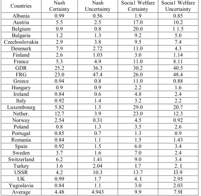
maximization). Looking at table 1 it can be seen that the Nash abatement rates are considerably

higher under uncertainty than under certainty for the USSR and FRG (more than twice as

much), and GDR; and somewhat higher for Bulgaria, Czechoslovakia, Italy, Poland, Romania,

Spain, Turkey, the UK and Yugoslavia.

Similarly, the social welfare solution is much higher under uncertainty than under

certainty for GDR and FRG, and somewhat higher for Turkey and USSR. The optimal

cooperative solution finds countries like Austria, Belgium, Bulgaria, Czechoslovakia, Greece,

Ireland, Luxembourg, Poland, Spain, USSR and the UK having to abate much more than the

amount of their Nash non-cooperative solution. On average, the Nash non-cooperative solution

under certainty is 4.5% while the social welfare solution is approximately 10%. These averages

are low because they rely on the existing secondary abatement in Europe in 1990. Although

secondary abatement takes place, in most of the other European countries secondary abatement

does not exist or it is very low.

From Tables 2 and 3 it can be seen that the Nash abatement costs are similar under

certainty and uncertainty for most European countries, except for the FRG (more than twice as

much), GDR and USSR but the Nash total damage costs are quite different (a result expected

according to the assumption of imperfect information regarding deposits). Under uncertainty

the main polluters (Eastern European countries, FRG, Ita1y, Spain, Turkey and the UK) abate

more. Countries receiving large amounts of sulphur deposits from others abate less: Austria,

Denmark, Luxembourg, Netherlands and the Scandinavian countries. The total damage costs

are higher under uncertainty on1y for the FRG, Poland, Spain, USSR, and the UK. For the rest

of the European countries the Nash damage cost is much lower under uncertainty.

In terms of totals, the Nash abatement costs are $884 m and $1037 m under certainty

and uncertainty respectively. As mentioned the increase in Nash abatement costs is carried

mainly by FRG, GDR and USSR. The Nash damage costs are $1229 m and $901 m under

certainty and uncertainty respectively. If countries cooperate then tota1 abatement cost is

$1006 m and $1078 m under certainty and uncertainty respectively. The abatement costs under

uncertainty are higher only for the FRG and Turkey. Besides, in terms of cooperative damage

costs we have $1063$ m and $851 m under certainty and uncertainty respectively.

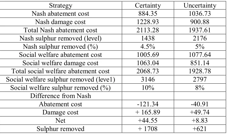
Finally, table 4 summarizes the results obtained by each strategy under certainty and

uncertainty for the year 2000. Ιt can be seen that, if countries cooperate under certainty they

will haνe to pay an extra 14% of the total Nash abatement cost. This will result in an extra 1.71

million tonnes of sulphur reduction and approximately 14% less damage cost. Similarly if

countries cooperate under uncertainty they will haνe to pay an extra 4% of the Nash total

abatement cost and this will reduce sulphur emissions by 621 million tonnes which is only one

uncertainty it can be seen that the Nash abatement costs are 17% higher under uncertainty and

Nash damage costs 27% higher under certainty.

It is notable that although for most countries the Nash abatement costs are simi1ar under

certainty and uncertainty, Germany (FRG and GDR) and USSR make the difference. If

countries cooperate then abatement costs are 7% higher and damage cost 20% lower under

uncertainty. But cooperation results in much higher abatement levels under certainty (1.7 m

tonnes) than under uncertainty (621 m t). Also the gains from cooperation are much higher

under certainty (45 m $) than under uncertainty (approximately 9 m $). Obviously, under the

assumption of stochastic deposits the gains from cooperation are much less than under the

assumption of deterministic deposits.

TABLE 1: Abatement rates under certainty and uncertainty (%)

Countries _Certainty Nash _Uncertainty Nash Socia1 Welfare _Certainty Socia1 Welfare _Uncertainty Albania 0.99 0.56 1.9 0.85 Austria 5.5 2.5 17.0 10.2 Belgium 0.9 0.8 20.0 1 1.5 Bulgaria 1.2 1.3 9.2 5.0 Czechoslovakia 2.9 3.8 9.5 7.4 Denmark 7.9 2.72 11.0 4.3 Finland 2.6 1.03 3.0 1.14

France 5.3 4.9 11.0 8.11 GDR 25.2 36.3 30.2 40.5 FRG 23.0 47.4 26.0 48.4 Greece 0.94 0.8 11.0 0.88 Hungary 0.9 0.9 2.2 1.6

Ireland 0.84 0.6 4.8 2.4 Italy 0.92 1.4 3.2 2.2 Luxembourg 5.82 1.5 29.0 20.7

Nether. 12.7 3.9 23.0 12.3 Norway 2.54 0.31 4.5 0.92 Poland 0.8 1.3 3.5 2.6 Portugal 0.85 0.7 1.3 0.9 Romania 0.84 1.1 1.5 1.43

TABLE 2: Total abatement costs under certainty and uncertainty forthe year 2000 (in 1985 $US m)

Countries _Certainty Nash _Uncertainty Nash Socia1 Welfare _Certainty Socia1 Welfare _Uncertainty Albania 0.0033 0.00102 0.0095 0.0023

Austria 0.173 0.33 2.035 0.525

Belgium 0.014 0.0098 10.3 2.23

Bulgaria 0.9266 0.93 1.3 1.011

Czechoslovakia 48.37 48.82 56.3 51.91

Denmark 0.73 0.074 1.5 0.185

Finland 16.17 16.065 16.2 16.07

France 38.79 38.321 47.3 41.38

GDR 134.43 143.0 168.9 158.06

FRG 101.64 245.33 135.2 255.49

Greece 17.65 17.645 17.67 17.65

Hungary 16.35 16.351 16.61 16.45

Ireland 0.0053 0.0027 0.184 0.042

Italy 100.5 100.66 101.93 101.063

Luxembourg 0.0144 0.001 0.65 0.1624

Netherlands 5.22 3.51 11.42 4.702

Norway 0.027 0.0004 0.088 0.0033

Poland 81. 15 81.3 82.91 82.01

Portugal 8.85 8.85 8.871 8.852

Romania 38.05 38.1 38.19 38.17

Spain 90.02 90.1 91.81 90.57

Sweden 0.118 0.02 0.4 0.046

Switzerland 0.434 0.02 1.0 0.1151

Turkey 38.32 38.46 38.34 38.471

USSR 0.43 2.38 5.66 4.323

UK 93.15 93.62 97.71 95.182

Yugoslavia 52.81 52.83 53.2 52.961

Total 884.35 1036.73 1005.69 1077.64

ΤABLE 3: Total damage costs under certainty and uncertainty for the year 2000 (in 1985 $US m)

Countries _Certainty Nash _Uncertainty Nash Socia1 Welfare _Certainty Socia1 Welfare _Uncertainty Albania 0.904 0.1251 0.87 0.122

Austria 11.773 0.9743 10.12 0.741

Belgium 3.198 0.9779 2.35 0.703

Bulgaria 0.765 0.3773 0.67 0.341

Czechoslovakia 41.5 29.53 36.13 27.077

Denmark 38.3 1.775 34.6 1.567

Finland 19.12 1.263 16.99 1.169

France 118.38 40.251 105.81 37.03

GDR 203.4 101.311 162.84 85.85

FRG 504.02 565.825 433.13 544.28

Greece 8.05 2.568 7.69 2.522

Hungary 10.98 4.971 10.37 4.83

Ireland 1.302 0.2934 1.22 0.274

Italy 20.06 19.51 18.96 19.083

Luxembourg 0.97 0.0365 0.713 0.0182

Netherlands 64.79 2.121 53.3 1.368

Norway 12.05 0.082 11.09 0.068

Poland 20.19 22.03 18.29 21.25

Portugal 3.05 0.919 2.94 0.903

Romania 11.87 8.863 11.33 8.722

Spain 5.83 6.329 5.32 6.032

Sweden 16.51 Ι. 184 15.03 1.094

Switzerland 39.83 0.842 36.48 0.711

Turkey 20.68 13.964 20.17 13.88

USSR 13.84 33.359 11.48 31.64

UK 30.23 36.035 28.231 34.84

Yugoslavia 7.34 5.361 6.92 5.22

TABLE 4: Abatement and damage costs (in US $m) and sulphur removed (in 1000 t)

Strategy Certainty Uncertainty

Nash abatement cost 884.35 1036.73

Nash damage cost 1228.93 900.88

Total Nash abatement cost 2113.28 1937.61

Nash sulphur removed (leνel) 1438 2176

Nash sulphur removed (%) 4.5% 5%

Social welfare abatement cost 1005.69 1077.64

Social welfare damage cost 1063.04 851.14

Total social welfare abatement cost 2068.73 1928.78

Social welfare sulphur removed (leνe1) 3146 2797

Social welfare sulphur removed (%) 10% 8%

Difference from Nash

Abatement cost -121.34 -40.91

Damage cost + 165.89 +49.74

Net +44.55 +8.83

Sulphur removed + 1708 +621

5. Summary and conclusions

In this paper, different equilibria concepts have been considered under the assumptions

of stochastic and deterministic sulphur deposits. One of the different equilibria was the Nash,

where each country minimizes only its own pollution control costs. But in global

environmental problems each country's own contribution to worldwide emissions is relatively

small so that there is little a country can do by itself. This interdependence across countries

provides a case for cooperation in sulphur emissions control policies (particularly in Europe),

since by cooperation of national policies a given set of deposition goals can be attained at a

lower cost than if each country acts in isolation. Distinguishing between certainty and

uncertainty about deposits, it was shown that:

1. Relying on the existing (if any) secondary abatement in Europe, it can be said that, in

order to achieve the environmental targets set by International Agreements (for

instance, "30% Club", "New Sulphur Protocol") it is required that countries will have to

use primary abatement. Targets less the optimal cooperative secondary abatement

high(6)_{. Otherwise, targets will not be satisfied (for more details see Halkos and Hutton,}

1994).

2. Under uncertainty the gains from cooperation are much less than under certainty.

3. Germany dominates the effort as its initial abatement is high. The old FRG has to abate

more than twice as much under uncertainty and it is the only country (except for USSR)

for which damage costs are higher under uncertainty. Additionally, a1though the Nash

abatement costs are similar under certainty and uncertainty Germany is again an

exceptional case.

4. The Nash abatement costs are similar under certainty and uncertainty for most countries

(except for GDR, FRG and USSR).

5. The Nash damage costs are quite different due το the assumption of stochastic deposits.

Under uncertainty countries wil1 face much less damage costs (except for FRG,

Poland, Spain, USSR, UK).

6. Main polluters abate more under uncertainty while pol1utees abate more under

certainty.

Finally, it is obvious that the nature of uncertainty matters. Here, a uniform probability

function was assumed for the deposits. This work can be extended by considering different

forms of probability density functions and their implications for the analysis. Also, an obvious

area for further research is how the change in European boundaries affects the results. It would,

however, be equally interesting to disaggregate the data to the levels of grids (squares) in order

to evaluate the consequences of local differences in either emissions or sensitivity το

depositions.

Acknowledgements

NOTES

(1) The estimates of the tonnes of sulphur emissions and the subsequent deposits between countries are based on the ΕΜΕΡ (1993) model (European Monitoring and Evaluation Program, Norwegian Meteorological Institute). The proportional transfer coefficients of the EMEP's transfer matrices have been used with IIASA's unconstrained sulphur emission estimates for the year 2000 (Amann and Sorensen, 1991) Το derive a transfer matrix of a closed system of 27 countries.

(2) The background deposits have been excluded as it is impossible to be tracked by our model.

(3) Other types of abatement options that are omitted in this approach are abatement through energy conservation in its broadest sense (energy demand suppression, fuel switching, and efficiency measures) and fuel substitution.

(4) For more details on the existing secondary abatement in Europe at 1990 and the future plans for installation of abatement technologies, see Halkos (1992) and Halkos and Hutton (1994). For the "New Sulphur Protocol" see Κlaasen (1993) and IIASA (1993).

(5) Originally, the model was estimated as ΤCabatement,i = a+diΤSRi+bi ΤSRi2. di was constrained

tο zero, however, for avoiding negative abatement solutions. Also, in the explicit set-up of the

model and for reasons of simplicity we preferred το use βi rather than all the monetary

coefficients a, di and bi. Obviously, after constraining di=0, βi ={[a/(αi2Ei2)]+bi}.

(6) Sulphur emissions can be reduced through either conservation or energy improvements. The latter can be achieved for instance by reducing energy consumption through more efficient generation, use of combined heat and power, etc. Low sulphur coal may be a good way to reduce emissions where emission standards are met by using coal within a specific range of

sulphur content. For instance, a standard of 2000 mg/m3 is equivalent to approximately 1%

sulphur content of coal, as the cut-off level above which sulphur abatement technologies would

be used. Emission standards between 1000 and 2000 mg/m3 _{are equivalent το coal sulphur}

REFERENCES

Αmann Μ. and Sorensen Ι., (1991). The energy and su1phur emission database of the RAINS

mode1, International Institute for Applied Systems, 46 pp.

Basar, Τ. & Olsder, G.J. (1982). Dynamic non-cooperative game theory. Academic Press,

London.

Bingham, G. (1986). Resolving environmental disputes: a decade of experience. Washingτon,

D.C.: Conservation Foundation.

Binmore, Κ. and Dasgupta, Ρ. (1990). The economics of bargaining. Basil B1ackwel1 Ltd.

ΕΜΕΡ (1993); Airborne transboundary transport of su1phur and nitrogen over Europe: model

description and calculations, Meteorological Synthesizing Centre-West, The Norwegian

Meteoro10gical Institute, EMEP/MSC-W Report 1/93 (Ju1y, 1993).

Halkos, G.E. (1992). Economic perspectives of the acid rain prob1em in Europe; D.Phil

Thesis, Department of Economics and Related Studies, University of York.

Halkos, G.E. (1993). Αn evaluation of the direct cost of abatement under the main

desu1phurization techno1ogies, Discussion Paper 9305, Department of Environmenta1

Economics and Environmenta1 Management, University of York.

Halkos, G.E. (1994); Optimal abatement of su1phur in Europe. Environmental and Resource

Economics, 4(2): 127-150.

Halkos, G.E. and Ηutton, J.P., (1993). Acid Rain Games in Europe; Discussion Paper 9312,

Department of Economics and Re1ated Studies, University of York.

Halkos, G.E. and Ηutton, J.P., (1994). Optimal acid rain abatement policy for Europe: an

analysis for the year 2000, Discussion paper 9403, Department of Environmental Economics

and Environmental Management, University of York.

Harisson, G.W. and Rutstrom, Ε.Ε. (1991). Trade wars, trade negotiations and applied game

theory. The Economic Journal, 101: 420-435.

Harsanyi, J.C. (1968). Games with incomp1ete information played by 'Bayesian' p1ayers parts

1, 2 and 3; Management Science, 14: 159-82, 320-34, 486-502.

Harsanyi J.C. and Selten, R. (1972). Α generalized Nash solution for two person bargaining

games with incomplete information. Management Science 18: 80-106.

Ηoel, Μ., (1991). Global environmenta1 prob1ems: the effects οf unilatera1 actions taken by

one country. Journa1 of Environmenta1 Economics and Management, 20: 55-70.

IlASA (1993). Options: IIASA's Project on Tranboundary Air Pollution. Internationa1 Institute

Κaitala, V., Pohjola, Μ. and Τahvonen, Ο. (1992). Transboundary Air Pollution and Soίl Acidification: a dynamic analysis of an acid rain game between Finland and the USSR.

Environmental and Resource Economics, 2(2): 167-181.

Klaasen, G., (1993). Trade-offs in emission trading, Paper presented at the Conference ''Economic Instruments for Air Pollution Control'', organized by the International Institute for Applied Systems, Laxenburg Austria, October 18-20.

Mäler, K.G. (1989). The acid rain game: valuation, methods and policy making in

environmental economics. In Valuation Methods and Policy Making in Environmental

Economics, edited by Η. Fo1mer and Ε. Ierland, Chapter 12.

Mäler, K.G. (1990). International environmental problems. Oxford Review of Economic Policy,

6(1): 80-107.

McDonald, Ι.Μ. and Solow, R.M. (1981). Wage bargaining and emp1oyment. American

Economic Review, 71: 896-908.

Μehimann, Α. (1988). Applied differential games. Plenum Press, ΝΥ, London.

Nash, J. (1950). The bargaining problem. Econometrica18: 155-62.

Nash, J. (1953). Two-person co-operative games; Econometrica21: 128-40.

Newbery, D. (1990). Acid rain. Economic Policy.

Raiffa, Η. (1953). Arbitration schemes for generalΊZed two person games. In Kuhm H.W. and

Tucker A.W. (eds.) Contributions to the Theory of Games II. Annals of Mathematics Studies

Νο 28, Princeton University Press.

Roth (1979). Axiomatic models of bargaining; Lecture notes in Economics and Mathematical

Systems Νο 170, Berlin: Springer-Verlag.

Shogren, J.F. and Crocker, T.D., (1991). Cooperative and non-cooperative protection against

transferable and filterable externalities. Environmental and Resource Economics, 1(1):

195-214.

Τahvonen, Ο., Κaitala, V. and Pohjola, Μ., (1993). Α Finnish-Soviet acid rain game: non-

cooperative equilibria, cost efficiency and su1phur agreements. Journa1 of Environmental

Economics and Management24: 87-100.

Vernon, J.L., (1989). Market impacts of sulphur contro1: the consequences for coal. ΙΕΑ Coal