Hybrid Feature based Natural Scene Classification using
Neural Network
Deepika Gupta
MITS Deemed University Lakshmangarh,
Rajasthan, India
Ajay Kumar Singh
MITS Deemed University Lakshmangarh, Rajasthan, India
Deepa Kumari
MITS Deemed University Lakshmangarh, Rajasthan, India
Raina
MITS Deemed University Lakshmangarh, Rajasthan, India
ABSTRACT
In this paper a classification for natural images is proposed using hybrid features. The objective of this paper is to develop an image content based classifier, which can perform identity check of a natural image. Here we have extracted wavelet and color features from a captured natural image to classify out of three groups. The developed technique is able to classify translation and rotation invariant matching among natural images using feed forward back propagation neural network. The database contains several hundreds of natural images of three groups namely coast, Forest, Mountain for classification and found good classification rate.
General Terms
Computer Vision, Pattern Recognition
Keywords
Neural Network, Statistical moment, Color Histogram, Hybrid Feature.
1.
INTRODUCTION
There are so many methods to classify natural scene images. Given a set of images of scenes is to classify a new image into one of these categories (e.g. coast, Forest, Mountains). One approach is to represent each of images by a vector and train neural network classifier on these vectors. There are so many approaches and techniques for improving classification accuracy [3, 4 and 5].
In image processing tasks texture analysis plays an important role, from remote sensing to medical Image processing, computer vision applications, and natural scenes. A number of texture analysis methods have been proposed [6]. Color is the most important property so performance of such methods can be improved by adding the color information, especially when dealing with real world images [7].
Wavelets are mathematical functions which help in describing the original image into an image in frequency domain. The wavelet features are extracted from original texture images and corresponding complementary images for texture classification [1]. Also the choice of filters in the wavelet transform plays an important role in extracting the features of texture images [11, 12].
An Artificial Neural Network (ANN) is an information processing system which is composed of a large number of highly interconnected processing elements (neurons) workings in unison to solve specific problems. In the work [2] different types of noise are classified using feed forward neural network.
They are usually used to model complex relationships between inputs and outputs or to find patterns in data [9, 11]. Constructive learning algorithms proposed an approach for the incremental construction of near-minimal neural-network architectures for pattern classification [19].
Recently, however, both color and texture information has been used by several researchers [7, 9].
In this paper, we use the Daubechies wavelet transform coefficients and color moments information as an input of NN. Color moments have been successfully used in many color based image classification systems, especially when the image contains just the object. Feed Forward NN (FFNN) with ten hidden layer is used in this paper for classification. Optimized methods with Momentum are used to learning the NN.
2.
2-D WAVELET TRANSFORM
A discrete wavelet transform (DWT) is any wavelet transform for which the wavelets are sampled discretely. Frequency and location information (location in time) both are captured by it. The transform is computed by applying a separable filter bank to the image:
A = [LX ∗ LY ∗ Im ↓2,1]↓1,2
H = [LX ∗ GY ∗ Im ↓2,1]↓1,2
V = [GX ∗ LY ∗ Im ↓2,1]↓1,2
D = [GX ∗ GY ∗ Im ↓2,1]↓1,2
where * denotes the convolution operator, ↓2,1(↓1,2) denotes the down sampling along the rows (columns) and Im is the original image, L and G are lowpass and highpass filters, respectively. Lowpass filtering generates A, is referred to as the low resolution image at scale one. Bandpass filtering is
done in a specific direction and thus contain directional detail information at scale one and generates H, V, D. The original image Im is thus represented by a set of sub images at several scales. Every detail subimage contains information of a specific scale and orientation. Spatial information is retained within the subimage. The basic idea of the wavelet transform is to represent any arbitrary function as a
superposition of wavelets. Any such superposition decomposes the given function into different levels, where each level is further decomposed with a resolution adapted to that level.
and down sampled by a factor of 2 in each direction, resulting in one low pass image LL and three detail images HL, LH, and HH. Figure 1 shows the one-level decomposition.
[image:2.595.325.487.78.242.2]LH channel contains image information of low horizontal frequency and high vertical frequency , HL channel contains high horizontal frequency and low vertical frequency , and the HH channel contains high horizontal and high vertical frequencies.
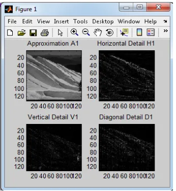
[image:2.595.84.253.185.249.2]Figure 1: 1-level Wavelet transform of 2D image
Figure 2: Wavelet Decomp. of a sample image
The frequency decomposition is shown in Fig. 1. Note that in multi-scale wavelet decomposition, only the LL sub band is successively decomposed.
3.
FEED FORWARD NEURAL
NETWORK
A neural network is a massively parallel distributed processor that has a natural propensity for storing experiential knowledge and making it available for use
.
Feed forward neural network begins with an input layer. This input layer must be connected to a hidden layer. This hidden layer can then be connected to another hidden layer or directly to the output layer. There can be any number of hidden layers so long as at least one hidden layer is provided. HereIi1,Ii2,…..Iin are the input neuron to the layerOo1……….OHm are output of hidden layer which gives
feedback to the output layer and Oo1,…….Oop are the output
of the output layers which are produce according to the activation function.
The activities of the neuron in input layer represent the raw information that is feed into the network.
Figure 4. Feed forward Network
Computation at Input Layer:
IHm =Oi1∗ W1m+ Oi2∗ W2m+ ⋯ Oin∗ Wnm…….(1)
Computation at Hidden Layer:
OHm=1+e−aIHm1 ……….(2)
The activity of the neuron in hidden layer is determined by the activities of the neurons in the input layer and the connecting weight between input and hidden neurons.
The activity of the output neurons depends on the activity of neurons in the hidden layer and the weight between the hidden and the output layer.
Computation at Output Layer:
IoP =OH1∗ W1P+ OH2∗ W2P+ ⋯ OHm ∗ WmP………(3)
OHm=1+e−aIOP1 ………...………(4)
Generally, the input layer is considered a distributor of the signals from the external world. Hidden layers are considered to be categorizers or feature detectors of such signals. The output layer is considered a collector of the features detected and producer of the response.
4.
HYBRID FEATURES
Since only RGB colors of the images will not be able to distinguish the different type of the image. Hence, hybrid feature is constructed by combining color moment feature of RGB, YCrCb, and HSV.
4.1
Color Moment Feature
Color images are represented in digital system by color intensity values of each pixel. These intensity values usually are described by three dimensional RGB color model as shown in the figure 5.
[image:2.595.79.252.282.470.2]Figure 5. RGB Color Model
The first order (mean=𝜇𝐾) the second order (variance=𝜎𝑘) and the third order moments (skewness=𝑆𝑘) of) color components are described through the following equations.
𝜇𝐾=𝑀𝑁1 𝑃𝑖,𝑗𝐾 𝑀
𝑗 =1 𝑁
𝑖=1
𝜎𝑘 = (𝑀𝑁1 (𝑃𝑖,𝑗𝑘 − 𝜇𝑘)2 𝑀
𝑗 =1
))
𝑁
𝐼=1
1 2
𝑆𝑘 = (𝑀𝑁1 (𝑃𝑖,𝑗𝑘 − 𝜇𝑘)3 𝑀
𝑗 =1
))
𝑁
𝐼=1
1 3
pI,JK is the value of the k-th color component of the image
ij-th pixel, and M is the height of the image, and N is the width of the image.
4.2
Daubechies Wavelet Feature
In this section we describe how wavelet features are extracted using DB4 wavelet. Due to the reason of important information is contained by the approximation coefficients, and hence they will constitute the part of extracted feature. However, obviously, there is also some important information in the high-frequency part. Hence, we are also considering high frequency coefficients. The information carried out by wavelet decomposed component’s moments have been proved to be efficient and effective in representing distributions of images [15]. Mathematically, the first three moments mean, variance and skewness are calculated from the individual coefficient matrix cA,cH,cV,cD.
5
METHODOLOGY:
Features are extracted by using given methodology. We are using two features of images that are RGB color values and wavelet coefficients using db4 wavelet decomposition. After that histogram are generated of these components to find out their statistical moments (mean, variance and first order moment). After applying this process we get 21 feature of each image((4 wavelet decomposition components like cA, cH, cV, cD+ 3 rgb component)* 3 features(mean, variance, skewness value)).
5.1
Data Set
Nine hundred sample images are taken from Oliva, Antonio Torralba database [23] with 300 sample each category mountains, cost and Forest. Each sample scene is shown in the fig 3.
Fig 3. Sample Images of coast, Forest, Mountain
5.2
Feature Extraction
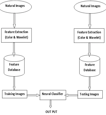
The feature extraction and classification process is shown through the figure 6. A database is created of different classes of image (coast, forest, mountains). Out of 900 sample images 300 images
are used to train the neural network and rest 600 images are used to test. Firstly images are resized to [256,256] and then converted to gray scale. After that image is decomposed using db4 wavelet transform which produces coefficients matrices cA, cH, cV, and cD (Approximation,
[image:3.595.86.219.86.199.2]Horizontal, Vertical, and Diagonal, respectively).
Figure 6. Feature extraction and classification
For signature or descriptive value we find the statistical moment up to 3 order moment of the coefficient matrices. Hybrid feature vector is prepared by finding the second feature color moment of the sample image, which are also described through statistical moment of RGB components extracted from the original image.
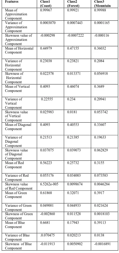
This process produces 21 signature values for each image. Feature vector for sample image of each category is shown in table 1. These features are arranged into a matrix. According to the combined color and texture feature, images database is created. After this network is trained using 100 images of each class. Thus 300 images are used to train the network and 600 to test the Network using feed forward Neural Network.
The classification is performed over a feed forward neural network model that consist of one input layer with five neurons, one hidden layer with ten neurons and one output layer with 3 neurons. Feed Forward Neural Network is used to train system, where the training dataset is constructed by
Natural Images
Feature Extraction (Color & Wavelet)
Feature Database
Training Images Neural Classifier
Natural Images
Feature Extraction (Color & Wavelet)
Feature Database
Testing Images
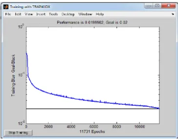
[image:3.595.324.502.346.539.2]the extracted features of the image. The entire input features are normalized into the range of [0,1], whereas the output class is assigned to one for the highest probability and zero for the lowest. The training performance graph is shown in the figure 7 with the goal 0.02.
6. EXPERIMENTAL RESULT
This section illustrates the result achieved in simulation of the test images. From the table 1 we can say that the system has shown the best performance for coastal images and comparatively weak for mountains. For the first category out of 200 samples 112 are classified correctly using RGB color feature, 176 are classified using db4 wavelet feature and 178 are classified using hybrid feature. Similarly for the forest images 140 are classified correctly using RGB color feature 138 are classified using db4 wavelet feature and 164 using hybrid feature. But in the third category out of 200 samples only 136 are classified using RGB color feature and 134 and 154 are by db4 and hybrid feature respectively. As shown in given below, table 1 shows Feature value of sample images.
[image:4.595.321.503.70.212.2]
Figure 2 shows comparitive classification rate using different feature, where A, B, and C is different category of images for Coast, forest and mountains respectively. Graph shows that classification rate fo costal images are high while weak for forest images.
Table 1: Classification rate for different feature set
S.NO. Image
Catagory RGB Color feature
db4 wavelet feature
Hybrid feature
1 Coast 56% 88% 89%
2 Forest 70% 69% 82%
3 Mountains 66% 64% 77%
Figure 8: Comparative classification rate using different
features
Figure 7: Performance graph of neural classifier
7. CONCLUSION
This work proposed an efficient signature based approach for natural image classification. Experimental result obtained using different features namely RGB color moment and db4 wavelet Transform feature and hybrid feature. In general, db4 gives better classification result but the combination of db4 wavelet feature and RGB color feature are more effective in scene classification. A feed forward neural network classifier is used to train network with sample pattern and shown the good results.
This work can further be extended by comparing with other features of image with different classifier e.g. nearest neighbor, SVM etc.
REFRENCES
[1] Ajay Kumar Singh, Shamik Tiwari, and V P Shukla, “Wavelet based multiclass Image classification using neural network”, International Journal of Computer Applications 37(4):21-25, January 2012.
[2] Shamik Tiwari, Ajay Kumar Singh and V P Shukla, “Statistical Moments based Noise Classification using
Feed Forward Back Propagation Neural
Network”, International Journal of Computer
Applications 18(2):36-40, March 2011.
[3] Anna Bosch, Xavier Munoz, Robert Martı.” A review: Which is the best way to rganize/classify images by content?”In Science Direct, Image and Vision Computing.12 july 2006.
[4]. Thyagarajan, K.S. Nguyen, T. Persons, C.E. Dept. of Electr. & Comput. Eng., San Diego State Univ., CA,” A maximum likelihood approach to texture classification using wavelet transform ”, Image Processing, 1994. Proceedings. ICIP-94., IEEE International .
[5] Abdulkadir sengur, “color texture classification using wavelet Transform and neural network ensembles”the arabian journal for science and engineering, volume 34, number 2b, february 9, 2009.
[6] J. Sklansky, “Image Segmentation and Feature Extraction”, IEEE Trans. System Man Cybernat., 8(1978), pp. 237–247.
[7] G. Van de Wouwer, P. Scheunders, S. Livens, and D. Van Dyck, “Wavelet Correlation Signatures for Color Texture Characterization”, Pattern Recognition, 32(3)(1999), pp. 443–451.
0% 20% 40% 60% 80% 100%
A B C
For RGB feature
For db4 wavelet feature
[image:4.595.75.302.365.617.2][8] A. Sengur, I. Turkoglu, and M. C. Ince, “Wavelet Packet Neural Networks for Texture Classification”, Expert Systems With Applications, 32(2)(2007), pp. 527–533.
[9] A. Sengur, “Wavelet Transform and Adaptive
Neuro-Fuzzy Inference System for Color Texture
Classification”, Expert Systems With Applications, 34(3)(2008), pp. 2120–2128
[10] I. Daubechies, “Orthogonal Bases of Compactly Supported Wavelets”, Comm. Pure. Appl. Math, 41(1988), pp. 909–996.
[11] Mojsilovic A., Popovic M.V. and D. M. Rackov, “On the selection of an optimal wavelet basis for texture characterization”, IEEE Transactions on Image Processing, vol. 9, pp. 2043–2050, December 2000.
[12] M. Unser, “Texture classification and segmentation using wavelets frames”, IEEE Transactions on Image Processing, vol. 4, pp. 1549–1560, November 1995.
[13] Rohit Arora et al. “An Algorithm for Image
Compression Using 2D Wavelet Transform”
International Journal of Engineering Science and Technology (IJEST), Vol. 3 No. 4 Apr 2011.
[14] M. Flickner, H. Sawhney, W. Niblack, J. Ashley, Q.Huang, B. Dom, M. Gorkani, J. Hafner, D. Lee, D.Petkovic, D. Steele, and P. Yanker, “Query by image and video content: The QBIC system.” IEEE Computer, Vol.28, No.9, pp.23-32, 1995.
[15] Stephane Mallat, A Wavelet Tour of Signal Processing. Academic Press, pp. 398-405, 1999.
[16]G.Pass,R.Zabih, and J.Miller. Comparing images using colr coherence vectors.InProceeding of 4th ACM International Confrence on multimedia,pages65-73, Bostan, Massachusetts, November 1996.
[17] B. Johansson , “A Survey on: Contents Based Search in Image Databases”, 2000.
[18] R.Duda,R.Hart, and D.Stark.Pattern Classification. John Wiley and sons.Inc,New York,2 edition,2000
[19] Henry A. Rowley, Shumeet Baluja, and Takeo Kanade,” Neural Network-Based Face Detection” PAMI, January 1998.
[20] A.k Jain,R.P.W. Duin and ,J.Mao.Stastistical Pattern Reconnition:A Review.IEEE Transaction on Pattern Analysis and Machine Intelligence,22(1)34-37,January 2000.
[21]. Parekh, R. Yang, J. Honavar, V.,” Constructive neural-network learning algorithms for pattern
classification” , IEEE Transactions on Neural
Network, Mar 2000,Vol. 11 ,No. 2,page(s): 436 – 451.
[22]J.Luo and A. Savakls.Indooe vs outdoor classification of consumer photograph using low level sementic feature.In IEEE International Confrences on Image Processing Thesanolnki,Grece,October 2001.
[23]
Aude Oliva, Antonio Torralba,”
Modeling the shape ofthe scene: a holistic representation of the spatial envelope”, International Journal of Computer Vision, Vol. 42(3): 145-175, 2001.
Table 2: Feature value of sample images.
Features Class1 (Coast)
Class2 (Forest)
Class3 (Mountain Mean of
Approximation Component.
0.99967 0.99921 0.99988
Variance of Approximation Component
0.0003070 0.0007443 0.0001165
Skewness value of Approximation Component
-0.000298 -0.0007222 -0.000116
Mean of Horizontal Component
0.44979 0.47155 0.36032
Variance of Horizontal Component
0.23038 0.23821 0.2084
Skewness of Horizontal Component
0.022578 0.013371 0.056918
Mean of Vertical Component
0.4093 0.46074 0.3689
Variance of Vertical Component
0.22555 0.234 0.20941
Skewness value of Vertical Component
0.025983 0.0181 0.053742
Mean of Diagonal Component
0.4093 0.40553 0.33607
Variance of Diagonal Component
0.21513 0.21385 0.19633
Skewness value of Diagonal Component
0.037075 0.039073 0.062829
Mean of Red Component
0.56223 0.25732 0.3155
Variance of Red Component
0.055176 0.034003 0.073583 Skewness value
of Red Component
6.5262e-005 0.0098674 0.0046284 Mean of Green
Component
0.61868 0.32071 0.3917
Variance of Green Component
0.049001 0.044933 0.021624 Skewness of Green
Component
-0.002860 0.011528 0.0018103 Mean of Blue
Component
0.6681 0.17943 0.39113
Variance of Blue Component
.0.070475 0.020213 0.0138 Skewness of Blue
Component
-0.011913 0.0050902 -0.0016891
[image:5.595.331.529.190.611.2]