Performance and Cost Benefit Analysis of a Hardware Software System Considering Hardware based Software Interaction Failures and Different Types of Recovery

Performance and Cost Benefit Analysis of a

Hardware-Software System Considering Hardware based Hardware-Software

Interaction Failures and Different Types of Recovery

Rajeev Kumar

Department of Mathematics, M.D. University, Rohtak-124001, INDIA

Monu Kumar

Department of Mathematics, M.D. University, Rohtak-124001, INDIA

ABSTRACT

In the present paper a hardware-software system that may have hardware, software and hardware based software interaction failures is taken. It is considered that a hardware and a software failure occurs purely due to respective hardware and software subsystems whereas a hardware based software interaction failure occurs whenever hardware degradation is not detected or repaired by the software method. It is assumed that, in addition to the software methods, recovery of the hardware and the software subsystems upon their failure may respectively be carried out by external hardware and software engineers. The measure of system performance such as mean time to system failure, expected up time of the system, expected down time due to pure hardware failure, expected down time due to pure software failure, expected down time due to hardware based software interactions failure, expected number of software repairs, expected number of hardware repairs, expected number of visits of hardware engineers, expected number of visits of software engineers, expected number of hardware repair by software method and expected number of software repair by re-execution are obtained using Markov process and regenerative point technique. Various conclusions regarding reliability and profit of the system are drawn on the basis of graphical studies.

General Terms

Stochastic Process

Keywords

Hardware-software system, Hardware based software interaction, MTSF, expected up time, expected down time, profit, Markov process, regenerative point technique

1.

INTRODUCTION

Almost all the modern systems like computers, mobiles, robots, missiles, rockets, radars etc. are nothing but hardware-software systems. A few of the numerous applications of these systems are control of communication and transport systems, automated plants operation, space explorations and even in routine activities of today society e.g., reservation of tickets, computation of various bills, in banks and in business, etc. All these things demand high reliability since failure of any can be costly and hazardous. As a hardware-software system means a system consists of two major components- hardware and software and therefore for effective performance of the system, both its hardware and software sub-components must function with considerable reliability. Even though these systems consists of hardware and software

subsystems, to judge reliability of the system, the researchers in the past dealt separately with hardware reliability and software reliability. For the reliability analyses of the whole system, combined reliability models, i.e. including both hardware and software subsystems were discussed by a few researchers such as Friedman and Tran [1], Hecht and Hecht [2], Kumar and Malik [3], Welke et al.[4], etc. assuming in general that these subsystem are independent of each other. That is, the aspects of interactions between the hardware and software subsystems were not taken up by them. However, Boyd et al.[5] discussed the difficulties in modeling hardware-software interactions.

Some researchers in the past including Iyer and Velardi [6], Martin and Mathur [7], Kanoun and Ortalo-Borrel [8], Haung et al.[9], justified that there exists remarkable interactions between hardware and software components. Therefore while developing combined reliability models the interactions between hardware and software components should not be ignored. Keeping this in view, Teng et al. [10] established a reliability modeling of the combined computer system by considering hardware, software and hardware based software interactions failures. Here the reliability of the combined system has been obtained by considering different models for hardware, software and hardware based software failure and not in fact in integrated way. Moreover various recovery aspects on different failures for the overall system have not been considered. To fill up this gap, recently a model for the whole computer system, i.e. including hardware, software and hardware based software interactions failures taking in to account different recovery aspects for the overall system has been developed by Kumar and Kumar [11] and discussed its reliability and availability.

In other words, it is considered that the system from its initial normal mode may go either to total hardware failures mode or to partial hardware (hardware degradation) mode or to total software failure mode. The repair at total hardware failure mode is carried out by the hardware engineer and the system reaches its normal mode whereas at total software failure mode repair is done by the software engineer. It is also assumed that from partial hardware mode system may go to software fail safe mode or to unsafe mode due to hardware-software interaction. The recovery from the fail safe to normal mode is possible by re-execution of the software whereas from fail unsafe mode to partial hardware failure mode through re-installation of the software by the software engineer. Other assumptions are:

1. The partial hardware failure may or may not be immediately detected. Once a partial hardware failure is detected, it can be recovered using software tool if not recovered using software method then hardware engineer is called to repair it.

2. An undetected degradation may cause a hardware related software failure (fail unsafe) mode and a detected degradation may cause an execution abortion (fail safe) mode.

3. On repair of the software in the safe mode the system recovers completely whereas on repair in the fail unsafe mode due to undetected hardware failure, the system is degraded.

4. All the failure and repair time distributions are exponential.

5. The external service facilities, i.e. hardware and software engineers, reaches the system in negligible time. 6. Switching is perfect and instantaneous.

7. All random variables are independent of each other.

The measures of system performance such as mean time to system failure (MTSF), expected up time, expected down time due to pure hardware failure, expected down time due to pure software failure, expected down time due to hardware based software interactions failure, expected number of software repairs, expected number of hardware repairs, expected number of visits of hardware engineers, expected number of visits of software engineers, expected number of hardware repair by software method and expected number of software repair by re-execution and profit are computed by making use of semi-Markov Process and regenerative point techniques. Various conclusions regarding reliability and profit of the system are drawn on the basis of graphical studies.

2.

NOTATIONS

1

h



: Hardware failure rate from normal mode to degradation partially failure mode.

2

h



: Hardware failure rate from partial hardware failure mode to total hardware failure mode.

3

h



: Hardware failure rate from normal mode to total hardware failure mode.

1

s



: Software failure rate from normal mode to total software failure mode.

2

s



: Software failure rate from undetected hardware partial failure mode to fail unsafe mode.

3

s



: Software failure rate from detected hardware partial failure mode to fail safe abortion mode.

1

p

: Probability that hardware degradation is detected.

1

q

: Probability that hardware degradation is not detected.

2

p

: Probability that hardware degradation is recovered by software methods.

2

q

: Probability that hardware degradation is not recovered by software methods.

1



: Hardware repair rate when degradation is detected and recovered by software methods.

2



: Hardware repair rate when degradation is detected and repaired by hardware engineer.

3



: Hardware repair rate of total hardware-software mode by the hardware engineer.

1



: Software repair rate on total software failure by the Software engineer.

2



: Software repair rate by the software engineer on fail unsafe mode.

3



: Software repair rate by the software engineer on fail safe mode.

3.

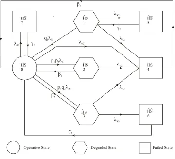
STATES OF THE SYSTEM

HS Normal mode.

ˆ

HS

Partial (degraded) hardware mode.

HS

Total (complete) hardware failed mode.

HS

Total (complete) software failed mode.

ˆ

HS

Fail unsafe mode.

ˆ

ˆ

HS

Fail safe mode.

The transition diagram showing the various states of the system is shown in the Fig.1. The epochs of entry into all the states are regenerative points and thus every state is regenerative state. The states 4, 5, 6 and 7 are the failed states.

4.

MEASURES

OF

THE

SYSTEM

PERFORMENCE

4.1

Transition Probabilities and Mean

Sojourn Time

The transition probabilities

p

_ijare given by:

01 1 2 h1

/

p



p p



S

p

₀₂



q

₁



h₁

/

S

03 1 2 h1

/

p



p q



S

p

₀₄





h₃

/

S

07 s1

/

p





S

p

₁₀





₁

/

S

₁

14 h2

/

1

p





S

p

₂₄





h₂

/

S

₂

25 s2

/

2

p





S

p

30





2

/

S

3

34 h2

/

3

p





S

p

₃₆





s₃

/

S

₃

40 52 60 70

1

p



p



p



p



Clearly, it can be verified that

01 02 03 04 07

1

p



p



p



p



p



p

10



p

14



1

24 25

1

p



p



p

₃₀



p

₃₄



p

₃₆



1

where

1 1 3

,

1 1 2

,

2 2 2

h s h h h s

S













S



 



S









and

3 2 s3 h2

Mean sojourn time

µ

_iin the

ith

state is the expected first

passage time taken by the

ith

state before transiting to any other state.

i

0

Pr( _i )

µ T t dt 







where

T

_i is the

p.d.f .

of device life time.

0

1/

S

 

,

 

₁

1/

S

₁,

 

₂

1/

S

₂,

 

₃

1/

S

₃

4 3

1







, 5 2

1







6 3

1







, 7 1

1







The unconditional mean time taken by the system to transition for any regenerative state j, when it (time) is counted from epoch of entrance into that state i is mathematically stated as:

*

0

( ) (0)

ij ij ij

m tq t dt q 







 

Thus,

2 01 1 2 h1/

m p p  S

2 0 2 1h /1

m  q S

, 2

03 1 2 h1/

m p q  S , 2

04 h3/

m  S

,

2 07 s1/

m  S

It is clear that

m

₀₁



m

₀₂



m

₀₃



m

₀₄



m

₀₇





₀ Similarly,

10 14 1

m



m





,

m

₂₄



m

₂₅





₂

30 34 36 3

m



m



m





_,

m

40





4 ,

52 5

m





,

m

₆₀





₆ and

m

₇₀





₇

4.2 Other Measures of System Performance

By probabilistic arguments for the regenerative process, we obtain the recursive relations for various measures of the system performance. On solving the recursive relations using Laplace and Laplace-Stieltjes transforms, we get the following measures in steady state:

Mean Time to System Failure 1

0

(T ) N D



Steady-State Availability ₀

1

(A ) N

D 

Expected Down Time due to

(a)Pure Hardware Failures (

DH

₀) = 2

1

N

D

(b)Pure Software Failures 3 0

1

(

DS

)

N

D



(c)Pure Hardware-Software Interaction Failures

4 0

1

(

DI

)

N

D



Expected Number of

(a) Software Repairs ₀ 5

1

(

RS

)

N

D



(b)Hardware Repairs 6 0

1

(

RH

)

N

D



(c) Hardware Repair by Software 9 0

1

(

HC

)

N

D



(d)Software Repair by Re-execution 10 0

1

(

SC

)

N

D



Expected Number of Visits by

(a)Hardware Engineer 7 0

1

(

VH

)

N

D



(b)Software Engineer ₀ 8

1

(

VS

)

N

D



Where

01 10 03 30

D 1

 

p p



p p

0 1 01 3 30 7 07

1 24 01 14 03 34

4 6 03 36

02 07

2 02 5 02 25

p

p

p

D

p

p p

p p

p p

p

p

p

p p

µ

µ

µ

µ

µ

µ

µ

µ



















_









_











_

_

_













24 0 1 01 3 30

2 02

N p p p

p

µ µ µ

µ

   



1

N





₀





_{1 01}

p





₂

p

₀₂





₃

p

₀₃





2 24 4 02 01 14 03 34

N



p

µ

p



p p



p p

3 24 07 7

N



p p

µ

4 02 25 5 24 03 36 6

N



p p

µ



p p p

µ

5 02 25 52 24 07 70

N



p p p



p p p





6 24 03 30 04 40

N



p

p p



p p





7 24 01 14 03 34 03 04 02 24

N



p

p p



p p



p +p



p p

8 02 25 07 24

N



p p



p p

9 01 10 24

N



p p p

10 03 36 24

N



p p p

5.

COST-BENEFIT ANALYSIS

The expected total profit

(P )

₀ incurred to the system in steady state is given by

0 0 0 1 0 0 0 2 0 3 0

4 0 5 0 6 0 7 0

P C A C (DH ) C RH C

C C C C _{h s}

DS DI RS

VH VS HC SC C C

      

    

where

0

C

= revenue per unit up time of the system.

1

C

= cost per unit down time of the system.

2

C

= cost per unit of hardware repair.

3

C

= cost per unit of software repair.

4

C

= cost per visit of hardware engineer.

5

C

= cost per visit of software engineer.

6

C

= cost per unit of the hardware repair by software.

7

C

= cost per unit of the software repair by re-execution.

h

s

C

= cost per unit of the software installation.

6.

PARTICULAR CASE

The values of the various failures rates and probability of hardware degradation detection as given in Teng et al. [10] and Trivedi et al. [12] i.e p1=0, p2=.95, q1=1, q2=.05, h1=.000526, h2=.000432, h3=.000112, s1=.000002, s2=.000263, s3=.00001, are taken as a particular case.

For this case values of various measures of system performance are computed from the results given in preceding section for assumed values of repair rates and various costs as

1=2, 2=.19, 3=.18, 1=0.8, 2=0.9, =5 C0 =25000, C1

=1000, C2 =500, C3 = C4 = C5 =200, C6 =500, C7 =200,

Ch =50000, Cs =150000. These values are as under:

Mean Time to System Failure = 3355.812

Steady-State Availability = 0.9989373

Expected Up Time =0.9989373

Expected Down Timedue to

(a) Pure Hardware Failures = 4.30395

(b) Pure Software Failures = .0058913

(c) Hardware based Software Interaction Failures = .0524048

Expected Number of

(a)Software Repairs =.05010978

(b)Hardware Repairs = .1649575

(c)Hardware Repair by Software = 0

(d) Software Repair by Re-execution = 0

Expected Number of Visitsby

(a)Hardware Engineer = .9396684

(b) Software Engineer =.05010978

Expected Profit = -154507.4

7.

GRAPHICAL ANALYSIS

For the analysis purpose various graphs are plotted for mean time to system failure and profit of the system for different values of hardware and software failures rates and probability of hardware degradation detection.

The behavior of MTSF with respect to various hardware failure rates h1, h2 and hardware based software failure rate s2 are depicted in Fig. 2 to Fig. 4. It can be observed from the

graphs that the MTSF decreases with the increase in the values of these failure rates. From Fig. 4, it can also be concluded that the MTSF increases with the increase in the values of the probability (p1) when other parameters remain

fixed.

Fig.5shows the pattern of the Profit (P0) with respect to the

software failure rate s2 for different values of hardware

failure rate h2. The profit (P0) decreases as the software

failure rate s2 increases and decreases for higher values of

software failure rate h2.

The curve in Fig. 6gives the pattern of the profit (P0) incurred

from the system with respect to the revenue per unit up time

(C0 h2. The

profit of the system increases as the revenue per unit up time (C0) increases whereas it decreases for higher values of h2. It can also be observed from the

graph that for h2 = 0.0002, P0 is positive if C0 >203694.036.

Therefore, the system is profitable whenever C0 >203694.036.

Similarly for h2 = 0.0006 and h2 = 0.001, the system is

profitable whenever C0>204099.85 and 204534.86

respectively.

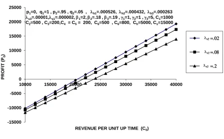
Fig.7 also reveals the pattern of the Profit (P0) with respect to

revenue per unit up time (C0) for different values of the

software s2. The profit (P0) increases as the

revenue per unit up time (C0) increases and decreases for

higher values of software the failure rate s2. It can also

observed from the graph that for s2 = 0.0001, P0 is positive if

C0 >203694.036. Therefore, the system is profitable whenever

C0 >203694.036. Similarly for s2 = 0.0006 and s2 = 0.0054,

the system is profitable whenever C0 >204099.85 and

204534.86 respectively.

8.

CONCLUSIONS

A stochastic model is discussed for hardware-software system considering hardware, software and hardware based software failures along with different recovery methods. The performance and cost-benefit analyses of the model are carried out. It is concluded that the reliability and profit of the system decreases with the increase in the values of pure hardware, pure software and hardware based software failure rates when other parameters are kept fixed. However, these increase with the increase in the probability of detection of hardware degradation. The limits for revenue up time, hardware and software failure rates are/ can be obtained for the system to give positive profit that may be quite useful for both the system engineer and the system user.

9. REFERENCES

[1] Friedman, M. A. and Tran, P., 1992. Reliability techniques for combined hardware/software systems, Proceeding Annual Reliability and Maintainability Symposium, pp.290-293

[2] Hecht, H. and Hecht, M., 1986. Software Reliability in the System Context, IEEE Transactions on Software Engineering, Vol.12, pp.51-58.

[3] Kumar, A. and Malik, S.C., 2012. Stochastic Modeling of a Computer System with Priority to PM over S/W Replacement Subject to Maximum Operation and Repair, International Journal of Computer Applications, Vol.43, No.3, pp. 27-34.

[4] Welke, S.R., Johnson, B.W. and Aylor, J.H., 1995. Reliability Modeling of Hardware/Software Systems, IEEE Trans. Reliability, Vol.44, pp.413-418.

[6] Iyer, R.K. and Velardi, P., 1985. Hardware related Software Errors: Measurement and Analysis. IEEE Transactions on Software Engineering, Vol.11, pp.223-230.

[7] Martin, R. and Mathur, A.P., 1990. Software and Hardware Quality Assurance: Towards a Common Platform for Increase the Usability of this Methodology, Proc. IEEE Conf. Comm.

[8] Kanoun, K. and Ortalo-Borrel, M., 2000. Fault-Tolerant Systems Dependability-Explicit Modeling of Hardware and Software Component-Interactions, IEEE Trans. Reliability, Vol. 49, No. 4, pp. 363-376.

[9] Huang, B., Li, X. , Li, M., Bernstein, J. and Smidts, C., 2005. Study of the Impact of Hardware Fault on Software Reliability, Proc. 16th IEEE International Symp. Software Reliability Engineering (ISSSRE’05).

[10]Teng, X., Pham, H. and Jeske, D.R., 2006. Reliability Modeling of Hardware and Software Interactions and its Applications, IEEE Trans. Reliability, Vol.55, pp.571-577.

[11]Kumar, R. and Kumar, M. 2011. Reliability and Availability Analysis of a Computer System with Hardware-Software Interactions and Different types of recovery, Proceeding of the International conference on Advances in Modeling, Optimization and Computing, I.I.T., Roorkee, pp.531-534.

[image:5.595.119.480.279.606.2]

[12]Trivedi, K. S., Vasireddy, R., Trindade, D., Nathan,S., and Rick Castro., 2006. Modeling High Availability Systems. Proceeding Pacific Rim Dependability Conference PRDC.

Fig.2

Fig. 3

0 100 200 300 400 500 600 700 800 900 1000

0 0.005 0.01 0.015 0.02

M

TSF

HARDWARE FAILURE RATE (h2)

MTSF VERSUS HARDWARE FAILURE RATE (h2) FOR

DIFFERENT VALUES OF HARDWARE FAILURE RATE (_h1)

 .01

.02

 .0

p1=0, q1=1, p2=.95, q2=.05, h3=.0000112,

_s1=.000002, _s2=.000263, _s3=.00001, 1=2, 2=.18, 3=.19, 1=1,2=1, 3=5

0 500 1000 1500 2000 2500 3000 3500 4000 4500

0 0.001 0.002 0.003 0.004 0.005 0.006

M

TSF

HARDWARE FAILURE RATE (h1)

MTSF VERSUS HARDWARE FAILURE RATE (_h1) FOR DIFFERENT VALUES OF HARDWARE FAILURE RATE (h2)

.001

.002

.00

p1=0, q1=1, p2=.95, q2=.05, h3=.0000112,

Fig.4

Fig. 5

0 1000 2000 3000 4000 5000 6000 7000 8000 9000 10000

0 0.2 0.4 0.6 0.8 1

M

TSF

PROBABILITY (p₁)

MTSF VERSUS PROBABILITY (p1) FOR DIFFERENT

VALUES OF HARDWARE FAILURE RATE (_h2)

0

.0005

.001

p2=.95,q2=.05,_h1=.000524,_h3=.000112, s1=.000002,s2=.000263,

s3=.00001,1=2, 2=.19, 3=.18, 1=0.8,

4430 4440 4450 4460 4470 4480 4490 4500

-0.001 0.001 0.003 0.005 0.007 0.009 0.011 0.013 0.015

PRO

FI

T

(P

0

)

SOFTWARE FAILURE RATE (s2)

PROFIT (P0) VERSUS SOFTWARE FAILURE RATE (s2) FOR

DIFFERENT VALUES OF HARDWARE FAILURE RATE (h2)

.01

.02

.0

p₁=.5, q₁=.95, p₂=.95, q₂=.05, _h1=.000526, _h3=.000263, _s3=.00001, s1=.000002, 1=2, 2=.18,3=.19,1=1,2=1,3=5,C0=25000,C1=1000,

Fig.6

[image:8.595.57.507.109.389.2]

Fig. 7

-15000 -10000 -5000 0 5000 10000 15000 20000 25000

10000 15000 20000 25000 30000 35000 40000

PRO

FI

T

(P

0

)

REVENUE PER UNIT UP TIME (C₀)

PROFIT (P₀) VERSUS REVENUE PER UNIT UP TIME OF THE SYSTEM (C0) FOR DFFERENT VALUES OF SOFTWARE FAILURE RATE (s2)

.02

.08

.2

p1=0, q1=1 , p2=.95 , q2=.05 , h1=.000526, h2=.000432, h3=.000263

s3=.00001,s1=.000002, 1=2, 2=.18 , 3=.19 , 1=1, 2=1 , 3=5, C1=1000

C₂=500 , C₃=200,C₄ = C₅ = 200, C₆=500 , C₆=800, C_h=5000, C_s=15000

-6000 -4000 -2000 0 2000 4000 6000 8000

198000 200000 202000 204000 206000 208000 210000 212000

PR

0

FI

T

(P

0

)

REVENUE PER UNIT UP TIME (C0)

PROFIT (P₀) VERSUS REVENUE PER UNIT UP TIME OF SYSTEM (C₀) FOR DIFFERENT VALUES OF HARDWARE FAILURE RATE (h2)

.0002

.0006

.0054

p₁=0, q₁=1, p₂=.95, q₂=.05, _h1=.000526, _s2=.0000112, _h3=.000263, s3=.00001, s1=.000002, 1=2, 2=.18, 3=.19, 1=1,2=1, 3=5,

C1=1000, C2=500,C3=200,C4 = C5=200, C6=500, C7=200,