http://dx.doi.org/10.4236/ijaa.2015.52013
Restricted Three Body Problem with Stokes
Drag Effect
Mamta Jain1, Rajiv Aggarwal2
1Department of Mathematics, Shri Venkateshwara University, Gajraula, India 2Department of Mathematics, Sri Aurobindo College, University of Delhi, Delhi, India Email: [email protected], [email protected]
Received 16 March 2015; accepted 8 June 2015; published 11 June 2015
Copyright © 2015 by authors and Scientific Research Publishing Inc.
This work is licensed under the Creative Commons Attribution International License (CC BY). http://creativecommons.org/licenses/by/4.0/
Abstract
The existence and stability of stationary solutions of the restricted three body problem under the effect of the dissipative force, Stokes drag, are investigated. It is observed that there exist two non collinear stationary solutions. Further, it is also found that these stationary solutions are unstable for all values of the parameters.
Keywords
Restricted Three Body Problem, Libration Points, Linear Stability, Dissipative Forces, Stokes Drag
1. Introduction
Two finite masses, called primaries, are moving in circular orbits around their common centre of mass, and an infinitesimal mass is moving in the plane of motion of the primaries. To study the motion of the infinitesimal mass is called the restricted three body problem. [1] proved that there existed five points of equilibrium, or points of libration (often denoted by L1, ….. L5), which were the stationary solutions of the restricted problem.
Out of them, three are collinear and two are non collinear. The collinear libration points are unstable for all val-ues of mass parameter µ and the triangular libration points are stable for 0< <µ µc, where µ =c 0.03852 is a critical value of mass parameter [2].
As we know, dissipative forces are those where there is a loss of energy such as friction and one of the most important mechanisms of dissipation is the Stokes drag which is a force experienced by a particle moving in a gas, due to the collisions of the particle with the molecules of the gas.
(
F Fx, y)
= −k x y(
− + Ωα y, y x+ − Ωα x)
where k∈
( )
0,1 is the dissipative constant, depending on several physical parameters like the viscosity of the gas, the radius and mass of the particle. Here( )
r r23 −Ω = Ω ≡
is the keplerian angular velocity at distance r= x2+y2 from the origin of the synodic frame and α∈
( )
0,1 is the ratio between the gas and keplerian velocities.A number of authors have investigated the location and stability of the equilibrium point in the presence of specific dissipative forces. [5] has used the Jacobi constant to investigate the effect of an external drag force proportional to the velocity in the rotating frame and has concluded that L4 and L5 are unstable to this type of
drag force. In their studies of the motion of dust particles in the vicinity of the Earth, [6] has analyzed the stabil-ity of the equilibrium points in the presence of radiation pressure which includes the Poynting Robertson drag terms. They have shown that the libration points are unstable to such a drag force. The effects of radiation pres-sure and Poynting Robertson light drag on the classical equilibrium points are analyzed by [7] and [8]. [9] has systematically discussed the dynamical effect of general drag in the planar circular restricted three body problem and has found that L4 and L5 are asymptotically stable with this kind of dissipation. It has been shown by [10],
[11], [12] and [13] that, in the case of Stokes drags, exterior resonances may compensate the decrease of the semi major axis and that stationary solutions still exist. A numerical analysis of 1:1 resonance, taking into ac-count the effect of the inclination and the eccentricity, has been studied by [14]. An analytical study of the linea-rised stability of L4 and L5 is provided in [4].
Furthermore, [15] has examined the linear stability of triangular equilibrium points in the generalized photo gravitational restricted three body problem with Poynting Robertson drag. They have considered the smaller primary as an oblate body and bigger one as radiating and they have concluded that the triangular equilibrium points are unstable in linear sense. [16] has discussed the nonlinear stability in the generalized restricted three body problem with Poynting Robertson drag considering smaller primary as an oblate body and bigger one ra-diating. They have proved that the triangular points are stable in nonlinear sense. [17] has discussed the stability of triangular equilibrium points in photo gravitational circular restricted three body problem with Poynting Ro-bertson drag and a smaller triaxial primary. They proved that the parameters involved in the problem (radiation pressure, oblateness and Poynting Robertson drag) influenced the position and linear stability of triangular points. In the presence of Poynting Robertson drag, triangular points are unstable, and in the absence of Poynt-ing Robertson drag, these points are conditionally stable. In a series of papers, [18] has performed an analysis in the restricted three body problem with Poynting Robertson drag effect. They found that there existed two non-collinear stationary solutions which were linearly unstable.
In the present paper, we study the same problem but with the effects of stokes drag instead Poynting Robert-son drag on noncollinear libration points L4 and L5 in the restricted three body problem.
2. Equations of Motion
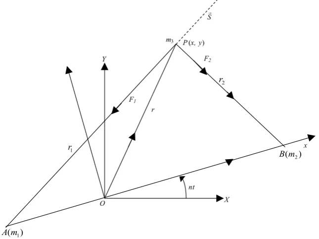
Suppose m1 and m2 are the primaries revolving with angular velocity n in circular orbits about their centre of
mass O, an infinitesimal mass
m
3 is moving in the plane of motion of m1 and m2. The line joining m1 and 2m is taken as X-axis and “O” their center of mass as origin and the line passing through O and perpendicular to OX and lying in the plane of motion of m1 and m2 is the Y-axis. We consider a synodic system of
coordi-nates O (xyz); initially coincident with the inertial system O (XYZ), rotating with the angular velocity n about Z-axis; (the z-axis is coincident with Z-axis) (Figure 1).
In the synodic axes the equation of motion of m3 in the restricted three body problem with Stokes drag Sis
(
)
2
3 2 2
m
t t t
∂ + ×∂ +∂ × + × × =
∂ ∂ ∂
r ω r ω r ω r ω F (1)
where
1 2 ,
= + +
Figure 1.Configuration of the restricted three body problem with Stokes drag S.
1
F = Gravitational Force acting on m3 due to 1 3 12 1 1
ˆ ,
m m
m G r
r =
2
F = Gravitational Force acting on m3 due to 2 3 22 2 2
ˆ ,
m m
m G r
r =
S = Stokes drags Force acting on m3 due to m1 along AP.
Its components along the synodic axes (x, y) are Sx =k x y
(
−)
+αS′y and Sy =k y x(
+)
−αS′x.where
( )
23,S′=S r′ =r−
,
OP xi yj
= = +
r n
= Κ =
ω Angular velocity of the axes O x y
( )
= const. The equations of motion of m3 in Cartesian coordinates (x, y) are(
)
(
)
(
)
1 2
1 2
2
1 3 2 3
2 y ,
x x x x
x ny n x Gm Gm Gk x y S
r
r
α− − ′
− − = − − − − +
(
)
1 2
2
1 3 2 3
2 y y x
y nx n y Gm Gm Gk y x S
r
r
α ′+ − = − − − + −
,
where
n = Mean motion, G = Gravitational constant,
(
x1,0)
and(
x2,0)
= coordinates of A and B in the synodic system.Using [2] terminology, the distance between primaries is unchanged and same is taken equal to one; the sum of the masses of the primaries is also taken as one. The unit of time is chosen so as to make the gravitational constant unity. The equations of motion of the infinitesimal mass m3 in the synodic coordinate system (x, y)
and dimensionless variables are
(
)
2 x y ,
x− y= Ω −k x y− +αS′
(2)
O X
x P(x, y)
Y
r
F2
m3
F1
nt
S
) (m1
A
) (m2
B
2
r
1
(
)
2 y x
y+ x= Ω −k y x+ −αS′
(3)
where
(
2 2)
(
)
1 2
1
1 ,
2 x y r r
µ µ
−
Ω = + + +
(
)
1
2 2
2 x y ,
r = +µ + (4)
(
)
2
2 2
2 x 1 y ,
r = + −µ + (5)
2
1 2
1 2
1 1 ; .
2
m m m
m m
µ= ≤ ⇒ = −µ =µ
+
The Stokes drag effect is of the order of k=10 ,−5 α =0.05 (generally k∈
( )
0,1 and α∈( )
0,1 as stated inthe introduction).
3. Stationary Solutions (Libration Points)
The solutions (x, y) of Equations (2) and (3) with x=0,y=0,x=0,y=0 are given by
(
) (
3)
(
3)
(
)
1 2
1
1 y 0,
x x
x k y S
r r
µ µ
µ + µ + − α ′
− − − + + = (6)
and
(
)
(
)
1 2
3 3
1
1 x 0
y k x S
r r
µ µ α
− ′
− − − − =
. (7)
Here, if we take k=0, then it will be the classical case of the restricted three body problem and the solutions of these equations are just the five classical Lagrangian equilibrium points Li (i = 1, 2, 3, 4, 5). The Li (i = 1, 2, 3) are three collinear libration points which lie along the x-axis and Li (i = 4, 5) are the two non collinear libration points which make the equilateral triangles with the primaries. Due to the presence of the Stokes drag force, it is clear from Equations (6) and (7) that collinear equilibrium solution does not exist. Since there is a possibility of non collinear libration points under the effect of drag forces, so we restrict our analysis to these points. Their lo-cations when k=0, are (see, e.g., [19])
4,5 0 12 , 0 23
L x = −µ y = ±
.
Now, we suppose that the solution of Equations (6) and (7) when k≠0 and y≠0 are given by
0 1, 0 2 1, 2 1
x x= +π y y= +π π π
Making the above substitutions in Equations (6) and (7), and applying Taylors series expansion around the li-bration points by using that
(
x y0, 0)
is a solution of these equations when k=0, we can get a linear set ofequations.
(
)
(
)
(
)
{
}
{
(
)
}
(
)
(
)
{
}
{
(
)
}
(
)
(
)
(
)
{
}
(
)
(
)
{
}
(
)
2 2
0 0
1 5 3 5 3
2 2 2 2 2 2 2 2 2 2 2 2
0 0 0 0 0 0 0 0
7
0 0 0 0 2 2 4
2 5 5 0 0 0 0
2 2 2 2 2 2
0 0 0 0
3 1 3 1 1
1 1
1 1
3 3 1 3
1 0
2 1
x x
x y x y x y x y
x y x y
k y x y y
x y x y
µ µ
π µ µ
µ µ µ µ
µ µ
π µ µ α
µ µ
−
+ + −
+ − − + −
+ + + + + − + + − +
+ + −
+ − + + + + =
+ + + − +
and
(
)
(
)
{
}
{
(
)
}
{
(
)
}
{
(
)
}
(
)
(
)
(
)
{
}
(
)
(
)
{
}
(
)
2 2 0 02 5 3 5 3
2 2 2 2 2 2 2 2 2 2 2 2
0 0 0 0 0 0 0 0
7
0 0 0 0 2 2 4
1 5 5 0 0 0 0
2 2 2 2 2 2
0 0 0 0
3 1 3 1
1 1
1 1
3 3 1 3
1 0
2 1
y y
x y x y x y x y
x y x y
k x x y x
x y x y
π µ µ
µ µ µ µ
µ µ
π µ µ α
µ µ − + − − + − + + + + + − + + − + + + − + − + − + + = + + + − + (9)
After substituting the values of the constants x0 and y0 in the above equations and rejecting the second
and higher order terms in π1 and π2, we get the values of π1 and π2 as
(
)
1 1 2 3 ,
2 3 k
π = − + α µ
(
)
2 185 2 3 k.
π = + α µ
Hence, putting the values of π1 and π2, the displaced equilibrium points are given by
(
)
(
)
4, 5 x 12 2 31 2 3 k y, 23 185 2 3
L = − −µ + α µ = ± + + α µk
(10)
Here, the shifts in L4 and L5 are of O k
(
µ)
. If we calculate(
x y,)
numerically, taking k=10 ,−5 α=0.05for different values of µ, we find that while using Stokes drag, as far as the values of µ increase corres-ponding x values decrease and the y values increase.
4. Stability of
L
4, 5We write the variational equations by putting x x= +ξ and y y= +η, ξ, η1, in the equations of mo-tion (2) and (3), where
(
x y,)
are the coordinates of the libration point. Therefore, expanding f x y(
,)
and(
,)
g x y by Taylors Theorem, we get
(
)
( )
(
)
( )
(
)(
)
( )
(
)
( )
(
)
(
)
( )
(
)(
)
( )
(
)
(
)
2 2 11
2 2 4
3 5 5 3
2 2 1 1
7 11
2 2 4 2 2 2 4
5 5
2 1
2
3 1 3 1 1 21
, 1
4
3 1 3 1 3 21 ,
2 4
x
x x x y
x y k x y k
r r r r
y x y x
k x y k y x y k
r r
ξ η
µ µ µ µ µ
µ α
ξ
µ µ µ µ
η α α
−
− −
−
+ − − + −
= Ω + − + + − − − +
+ − − + + + + + + − + (11)
(
)
(
)
( )
(
)(
)
( )
(
)
(
)
( ) ( )
(
)
( )
(
)
( )
(
)
7 112 2 4 2 2 2 4
5 5
2 1
2 11
2
2 2 4
5 2 5 3
2 2 1 1
2
3 1 3 1 3 21
,
2 4
3 1 1
3 21
1 .
4 y
y x y x
x y k x y k x x y k
r r
y
y k x y x y k
r r r r
η ξ
µ µ µ µ
ξ α α
µ µ
µ µ α
η
− −
−
+
+ − − +
= Ω + + − − + + +
− − + + − + − − + + (12)
Let us consider the trial solution of Equations (11) and (12),
0e ,λt 0eλt ξ ξ= η η=
( )
(
)
( )
(
)(
)
( )
(
)
( )
(
)
(
)
( )
(
)(
)
( )
(
)
(
)
2 0 02 2 11
2 2 4
0 3 5 5 3
2 2 1 1
7 11
2 2 4 2 2 2 4
0 5 5
2 1
e 2 e
3 1 3 1 1 21
e 1
4
3 1 3 1 3 21
e ,
2 4
t t
t
t
x x k x y x y k
r r r r
y x y x
k x y k y x y k
r r
λ λ
λ
λ
λ ξ λη
µ µ µ µ µ
µ α
ξ λ
µ µ µ µ
η λ α α
− − − − + − − + − = − + + − + − + + − − + + + + + + − + (13)
(
)
( )
(
)(
)
( )
(
)
(
)
( ) ( )
(
)
( )
(
)
( )
(
)
2 0 0 7 112 2 4 2 2 2 4
0 5 5
2 1
2 11
2
2 2 4
0 5 2 5 3
2 2 1 1
e 2 e
3 1 3 1 3 21
e
2 4
3 1 1
3 21
e 1 .
4
t t
t
t
y x y x
k x y k x x y k
r r
y
y k x y x y k
r r r r
λ λ
λ
λ
λ η λξ
µ µ µ µ
ξ λ α α
µ µ
µ µ α
η λ − − − + + − − + = + − − + + + − − + + − + − − + + (14)
Now, from Equations (13) and (14), we derive the following simultaneous linear equations
( )
(
)
( )
( )
(
)
( )
(
)
(
)
( )
(
)(
)
( )
(
)
(
)
2 2 11
2 2 2 4
3 2 3 2
1 1 2 2
7 11
2 2 4 2 2 2 4
5 5
2 1
3 3 1
1 1 1 1 21
4
3 1 3 1 3 21
2 0
2 4
x x k x y x y k
r r r r
y x y x
k x y k y x y k
r r
µ µ
µ µ α
ξ λ λ
µ µ µ µ
η λ λ α α
− − − − + + − + − + − − − + + + − − + + − − − − − + − + = (15) and
(
)
( )
(
)(
)
( )
(
)
(
)
( )
( )
( )
( )
(
)
7 112 2 4 2 2 2 4
5 5
2 1
11
2 2
2 2 2 4
3 2 3 2
1 1 2 1
3 1 3 1 3 21
2
2 4
1 1 3 1 3 1 21 0
4
y x y x
k x y k x x y k
r r
y y k x y x y k
r r r r
µ µ µ µ
ξ λ λ α α
µ µ α
η λ λ
− − − + − − + − − + + + − + − + + − + − − − − + = (16)
The simultaneous linear Equations (15) and (16) can be written as
(
2)
(
)
, , ,
1 x x x x 2 x y 0
e h k k g k
ξ λ + − − −λ − +η − λ− − = (17)
(
)
(
2)
, , ,
2 g ky x e f 1 ky y ky y 0
ξ λ− + +η λ + − − −λ − = (18) where
( ) ( )
3 31 2 1 , e r r µ µ −
= + (19)
( ) ( )
5 5 21 2 1 3 , f y r r µ µ − = +
(20)
(
)(
)
( )
(
)
( )
5 5 1 2 1 13 x x ,
g y
r r
µ µ µ µ
− + + −
= +
(21)
(
)(
)
( )
(
)
( )
2 2 5 5 1 2 1 13 x x .
h
r r
µ µ µ µ
− + + −
= +
(22)
(
)
(
)
(
)
11
2 2 4
, ,
11
2 2 2 4
,
11
2 2 2 4
, , ,
2 ,
21 , ,
4
21 ,
4
21
0, , 0,
4 21
4
x x
x x x x
x x y
y y
x
x y y x y x
y y y
S S
k x y x y k k k
x x
S
k k y x y k
y
S S
S
k k k x x y k k
y x x
S k x y α α α α − − − − − − − − − − ∂ = = + = = ∂ ∂ ∂ = = − + + ∂ ∂ ∂ ∂ = = = = + + = = ∂ ∂ ∂ ∂ = ∂ = +
(
2)
411,
, y .
y y S
y x y k k k
y − − ∂ = ∂ = (23)
Neglecting terms of O k
( )
2 , the condition for the determinant of the linear equations defined by theEqua-tions (17) and (18) to be zero is
(
)
(
)
(
)
(
)
(
)
(
) (
)
(
)(
) ( ) (
)
(
)
(
)
4 3 2
, , , , , ,
, , , , , ,
2
, , , ,
2 1 2
1 1 2
1 1 1 1 0
x x y y x x x y y x y y
x x y y x y y x x y y x
x x y y x y y x
k k e f h k k k k
e f k e h k k k g k k
e h e f g e f k e h k g k k
λ λ λ
λ − + + + − − − + − − + − + + − + + − − + + − − − − − + − + + − + − + = (24)
This quadratic Equation (24) has the general form
(
)
(
)
4 3 2
3 20 2 1 00 0 0
λ +σ λ + σ +σ λ +σ λ+ σ +σ = (25)
where
(
)
(
)
(
)
0 1 e f kx x, 1 e h ky y, f kx y, ky x, ,
σ = − + + − + − +
(
)
(
)
(
)
1 1 e f kx x, 1 e h ky y, 2 kx y, ky x, ,
σ = − + + − + + −
2 ky y, kx x, , σ = − −
3 kx x, ky y, , σ = − −
(
)
20 2 1 e f h,
σ = + − −
(
)(
)
200 e f 1 e f 1 g .
σ = − − − − −
Here σ00, σ20 and σi
(
i=0,1,2,3)
can be derived by evaluating e, f, g and h defined earlier. The value ofthe coefficient in the zero drag case is denoted by adding additional subscript 0. If we neglect product of powers of µ with any of the constants defined in Equation (23), we obtain
(
)
(
)
(
)
(
)
(
)
(
)
(
)
00 20
11 11 7 7
2 2 4 2 2 4 2 2 4 2 2 4
0
11 11
2 2 2 4 2 2 2 4
1
11
2 2 4
2 3
27 , 4 1,
189 63 63 3 63 3 ,
16 16 16 8
21 21 1 , 2 2 21 , 2 2 .
x y x y k x y x y k x y x y k
x x y y x y k
x y x y k
k
σ µ
σ
α α α α µ
σ
σ α α
σ α σ − − − − − − − = = − = + − + + + − + = − + + − + = − + = − (26)
4 2
20 00 0
λ +σ λ +σ = (27)
The four classical solutions for L4 and L5 to O
( )
µ are given by the pair of values4,5 1,2
3,4
27
: 1
4 27
4
L λ µ
λ µ
= ± − +
= ± −
(28)
Since we are primarily interested in the stability of L4 and L5 under the effects of a drag force, we restrict our
analysis to these points. The four roots of the classical characteristic equation can be written as
( 1, ,4)
n i n
λ = ± Τ = (29) where
2
20 20 4 00
2
σ ± σ − σ
Τ = (30)
is a real quantity for L4and L5. Using the values of σ00 and σ20 given in Equations (26) we have
2 1 27 or 2 27
4 µ 4 µ
Τ = − Τ = (31)
With the introduction of drag we assume a solution of the form
(
1)
(
1)
n i i
λ λ= + +ρ υ =∓υ± +ρ Τ (32) where ρ and υ are small real quantities. To lowest order we have
(
)
2 1 2 2 i 2
λ = − + ρ − υ Τ (33)
(
)
3 3 1 3 i 3
λ = ± υ∓ + ρ Τ (34)
(
)
4 1 4 4 i 4
λ = + ρ + υ Τ (35)
Substituting these in Equation (25), and neglecting products of ρ or υ with σi, and solving the real and imaginary parts of the resulting simultaneous equations for ρ or υ we get
(
)
2
3 1
2 20
, 2 2
σ σ
υ
σ
± Τ =
Τ Τ −
∓ (36)
(
) (
)
(
)
2 4
00 0 20 2
2 2
20
.
2 2
σ σ σ σ
ρ
σ
+ − + Τ + Τ
=
Τ − Τ (37)
(i) The stability of L4
For L4, we have
(
)
2
3 1
2 20
, 2 2
σ σ
υ
σ
Τ − =
Τ Τ − (38)
(
) (
)
(
)
2 4
00 0 20 2
2 2
20
.
2 2
σ σ σ σ
ρ
σ
+ − + Τ + Τ
=
Τ − Τ (39)
On putting the values of σi, in Equations (38) and (39) from Equation (26) and also taking, Τ =2 274 µ, we have
27
, .
8 108 3 3
k µ
υ ρ
µ µ
= =
Now, putting these values of ρ and υ in Equation (35), and neglecting the terms of O k
( )
µ , we get the characteristic equation as2
4 729 0
16 216
µ λ
µ
− =
−
whose roots are
(
)
(
)
(
)
(
)
1 3 1 2 3 1
4 4 4 4
3 3 1 4 3 1
4 4 4 4
3 3 , 3 3 ,
2 2 27 2 2 27
3 3 , 3 3 .
2 2 27 2 2 27
i
i
µ µ
λ λ
µ µ
µ µ
λ λ
µ µ
= − = −
− −
= =
− −
Also on taking 2 1 27
4 µ
Τ = − in Equations (38) and (39) from Equation (26), we get the characteristic equa-tion as
(
)(
)
(
)
4 4 27 4 81 0
8 2 27 ik
µ µ
λ
µ
− + − +
+ − =
− +
whose roots are
(
)
(
)
(
)
(
)
(
)
(
)
(
)
(
)
1 3 1 2 3 1
4 4 4 4
2
3 3 1 4 3 1
4 4 4 4
16 432 16 16 432 16
, ,
2 2 27 2 2 27
16 432 16
16 432 16
, .
2 2 27 2 2 27
i k i k
i k
i k
µ µ
λ λ
µ µ
µ µ
λ λ
µ µ
− + − − + +
= − = −
− + − +
− + −
− + +
= =
− + − +
If υ ≠0,
According to [9], the resulting motion of a particle is asymptotically stable only when all the real parts of λ
are negative and the condition for asymptotically stable under the arbitrary drag force is given by
1 3
0<σ <σ (40) where σ1 and σ3 are defined in Equation (26). But we see that the linear stability of triangular equilibrium
points does not depend on the value of kx x, and ky y, . Therefore the condition σ >3 0 can only be satisfied
when k is positive and the drag force is a function of x and y.
But here in our case of Stokes drag σ1= −k,σ3= −2k and therefore σ1 >σ3 and henceL4 is not
asymp-totically stable. Further one of the roots of λ i.e. λ4 has positive real root. Therefore L4 is not stable. Thus we
conclude that L4 is neither stable nor asymptotically stable and hence linearly unstable.
Similarly, we conclude that L5 is neither stable nor asymptotically stable and hence linearly unstable.
5. Conclusions
We have studied the existence of the triangular libration points and their linear stability by using Stokes drag. We have shown that there exist two noncollinear stationary points L x y4
(
,)
and L x y5(
,−)
(Equation (10)).If we put k=0, these results agree with the classical restricted three body problem.
In the classical case i.e. when k=0, we observe that as the value of µ increases, the abscissa x of L4
decreases and the ordinate y of L4 remains constant, while in our case (i.e. Stokes drag), when k=10−5, we
observe that the abscissa x of L4 decreases and the ordinate y of L4 changes slightly. In our previous
paper ([18]) i.e. in the case of Poynting Robertson drag, the abscissa and the ordinate decrease with µ. As re-gards, the stability of L4 in both the cases (Poynting Robertson drag and Stokes drag) is always unstable for all
In the case of Stokes drag, we have derived a set of linear equations in terms of ξ and η (Equations (17) and (18)), which involve the components of the Stokes drag force evaluated at the libration points (Equations (19)-(23)). From these, we derive a characteristic equation having the general form (Equation (25)).
Further, we have derived the approximate expressions for σ σ σ σ σ0, , , ,1 2 3 00 and σ20 occurring in the above
characteristic equation. These expressions are given in terms of the partial derivatives of the Stokes drag, eva-luated at the libration points.
Using the [9] terminology, in the case of drag force, we assume a solution of the form (Equation (32)), where
υ and ρ are small real quantities and
(
1, ,4)
n i n
λ = ± Τ =
is a real quantity for L4and L5 in the classical case. After substituting the values of λ, λ2, λ3 and λ4 in the
characteristic equation, we get the values of υ and ρ (Equations (36) and (37)).
Further to investigate the stability of the shifted points, by using [9] terminology, the resulting motion of a particle is asymptotically stable only when all the real parts of λ are negative. Also, the condition for asymp-totical stability under the drag force is given by Equation (40).
The condition σ >3 0 can only be satisfied when k > 0. In the case of Stokes drag σ = −1 k and σ = −3 2k,
Equation (40) is not satisfied. Therefore, L4and L5 are not asymptotically stable. Further, we have seen that one
of the roots of λ i.e. λ4 has positive real root; thus, L4and L5 are not stable. Hence, due to Stokes drag, L4
and L5 are neither stable nor asymptotically stable but unstable whereas in the classical case L4and L5are stable
for the mass ratio µ<0.03852 [19].
References
[1] Euler, L. (1772) Theoria Motuum Lunae, Typis Academiar Imperialis Seientiarum, Petropoli. Reprinted in Opera Om-nia, Series 2, Courvoisier, L., Ed., Vol. 22, Orell, Fussli Turici, Lausanjse, 1958.
[2] Szebehely, V. (1967) Theory of Orbits, the Restricted Problem of Three Bodies. Academic Press, New York and Lon-don
[3] Celletti, A., Stefanelli, L., Lega, E. and Froeschlé, C. (2011) Some Results on the Global Dynamics of the Regularized Restricted Three-Body Problem with Dissipation. Celestial Mechanics and Dynamical Astronomy, 109, 265-284. http://dx.doi.org/10.1007/s10569-010-9326-y
[4] Murray, C.D. and Dermott, S.F. (1999) Solar System Dynamics. Cambridge University Press, Cambridge. [5] Jeffreys, H. (1929) The Earth. 2nd Edition, Cambridge University Press, Cambridge.
[6] Colombo, G.D., Lautman, I. and Shapiru, I. (1966) The Earth’s Dust Belt: Fact or Fiction? Gravitational Focusing and Jacobi Capture. Journal of Geophysical Research, 71, 5705-5717. http://dx.doi.org/10.1029/JZ071i023p05705
[7] Schuerman, D. (1980) The Restricted Three-Body Problem Including Radiation Pressure. Astrophysical Journal, 238, 337-342. http://dx.doi.org/10.1086/157989
[8] Simmons, J.F.L., Mcdonald, A.J.C. and Brown, J.C. (1985) The Restricted Three-Body Problem with Radiation Pres-sure. Celestial Mechanics, 35, 145-187. http://dx.doi.org/10.1007/BF01227667
[9] Murray, C.D. (1994) Dynamical Effects of Drag in the Circular Restricted Three Body Problems: 1. Location and Sta-bility of the Lagrangian Equilibrium Points. Icarus, 112, 465-184. http://dx.doi.org/10.1006/icar.1994.1198
[10] Beauge, C. and Ferraz-Mello, S. (1993) Resonance Trapping in the Primordial Solar Nebula: The Case of a Stokes Drag Dissipation. Icarus, 103, 301-318. http://dx.doi.org/10.1006/icar.1993.1072
[11] Beauge, C. and Ferraz-Mello, S. (1994) Capture in Exterior Mean Motion Resonance Due to Poynting Robertson Drag.
Icarus, 110, 239-260. http://dx.doi.org/10.1006/icar.1994.1119
[12] Beauge, C., Aarseth, S.J. and Ferraz-Mello, S. (1994) Resonance Capture and the Formation of the Outer Planets.
Monthly Notices of the Royal Astronomical Society, 270, 21-34. http://dx.doi.org/10.1093/mnras/270.1.21
[13] Sicardy, B., Beauze, C., Ferraz-Mello, S., Lazzaro, D. and Roques, F. (1993) Capture of Grains into Resonances through Poynting-Robertson Drag. Celestial Mechanics & Dynamical Astronomy, 57, 373-390.
http://dx.doi.org/10.1007/BF00692487
[14] Liou, J.C., Zook, H.A. and Jackson, A.A. (1995) Radiation Pressure, Poynting Robertson Drag and Solar Wind Drag in the Restricted Three Body Problem. Icarus, 116, 186-201. http://dx.doi.org/10.1006/icar.1995.1120
http://dx.doi.org/10.1080/1726037X.2006.10698504
[16] Kushvah, B.S., Sharma, J.P. and Ishwar, B. (2007) Nonlinear Stability in the Generalised Photogravitational Restricted Three Body Problem with Poynting-Robertson Drag. Astrophysics and Space Science, 312, 279-293.
http://dx.doi.org/10.1007/s10509-007-9688-0
[17] Singh, J. and Emmanuel, A.B. (2014) Stability of Triangular Points in the Photogravitational CR3BP with Poynting Robertson Drag and a Smaller Triaxial Primary. Astrophysics and Space Science, 353, 97-103.
http://dx.doi.org/10.1007/s10509-014-2023-7