Solving Linear Systems of Equations using a
Memetic Algorithm
Liviu Octavian Mafteiu-Scai
West University of Timisoara, Timisoara, Romania
Emanuela Jana Mafteiu-Scai
National College „Iancu de Hunedoara”, Hunedoara, Romania
ABSTRACT
This paper proposes a memetic algorithm (MA) to solve linear systems of equations, by transforming the linear system of equations into an optimization problem. Such exploitation of knowledge obtained in a local search/optimization allows the evolutionary programming implementation to produce very good results at a relatively low computational cost. The proposed MA is able to determine solutions of a given linear system of equations, even in cases where traditional methods fail ( determinant null, ill-conditioned systems, subdeterminate systems, supradeterminate systems, system doesn’t satisfy the convergence conditions etc). In situations when a linear system of equations has multiple solutions, in proposed approach, the task is to find as many solutions as possible, inside of a given interval. In cases where no accurate solution for a linear system of equations exists, an approximate solution can be acceptable and it can be obtained by the proposed method.
General Terms
Algorithms.
Keywords
linear systems of equations, memetic algorithms
1. INTRODUCTION
1.1 Solving systems of linear equations
A frequent problem in numerical analysis is solving the linear systems of equations. That, consequently has generated a great interest among mathematicians and computer scientists, as evidenced by the large number of numerical methods developed over time. Besides the classical numerical methods, recently were proposed methods inspired by techniques from artificial intelligence. Hybrid methods have been also proposed along the time.
The classical methods are usually divided into exact/direct methods and iterative/indirect methods. In direct methods, the solution is obtained after a fixed number of operations, a number that is directly proportional to system size. In this case the solution is only affected by rounding errors and are preferred when the size of the system is acceptable. The most known direct methods are: Cramer, Gaussian elimination, Gauss-Jordan elimination, LU factorization, QR decomposition etc. In indirect methods the iterative process will be stopped after a preset number of steps or after fulfilling certain conditions. The process involves iterative appearance of truncation errors, the main disadvantage of these methods. However, because the rounding errors are not cumulated and because requiring a smaller number of operations, iterative methods are preferred especially for large
systems of equations. The most known are: Gauss-Seidel method, Jacobi method, gradient and conjugate gradient methods, etc. The literature describing the classical methods is more than rich. As mentioned, for solving linear systems of equations there are known a lot of algorithms. But in the cases of general n x m matrices, when n<m (m is the number of unknown variables and n is the number of equations) the classical iterative algorithms are not applicable, with a few exceptions.
In the last years, techniques and methods from the field of artificial intelligence have been used to solve or preconditioning solving the systems of equations. In [1] is proposed an algorithm that uses a genetic approach to solve linear systems of equations. This problem is viewed in terms of an optimization task. There is defined a cost function with interval variables that is further minimized. The cost function used in the genetic algorithm is
g = max [abs(fi)] for i =1,2,3,…,n where max [abs (fi)] is the maximum absolute value of individual equations
fi(x) = 0 of a system, with n such equations. In [2], the authors investigate the applicability and effectiveness of genetic algorithms in finding the solutions of systems of linear equations. Solving a system of equations is regarded again as an optimization problem. The proposed algorithm is able to produce more than one set of solutions for a systems of equations. In that approach a chromosome is represented by a vector with integer values that corresponds to the unknowns of the system. The crossover and mutation operation are used in solving process. In terms of the objective function, the approach is similar to that in [1], but the problem is interpreted as a multiobjective optimization task. Such a multiobjective optimization approach is not new, since similar approaches were proposed also in [3, 4, 5, 7]. In [6], the proposed method for solving a linear system of equations is based on using a particle swarm optimization algorithm and an artificial fish swarm algorithm, especially designed for ill-conditioned linear systems equations.
1.2 Memetic algorithms and optimization
problems
view, the MAs are population-based metaheuristics. A reference book that makes a detailed description of memetic algorithms is [8]. An extensive description of other nature-inspired intelligent algorithms can be found in [9, 10, 11, 12]. The general structure of MA is presented in Algorithm 1 Algorithm 1:
Begin
Initialize Population Repeat
Evaluate Curent Population Select Parents
Crossover Mutation
Evaluate New Chromosomes Improve With Local Search
If Converged then Restart Population Until TerminationCriterium
End
Some aspects are very important in terms of designing a good memetic algorithm:
- the choice of recombination operators in the evolutionary process must take into consideration the three basic properties of these: purity, assortment and transmission [10];
- a clear separation between local search/optimization and global search/optimization must be made. At the same time a balance between local and global search is required to avoid premature convergence and the waste of computing resources; - in case of population convergence, the population must be refreshed in order to avoid the exploration of the same search space, which would lead to obtaining the same solutions and unnecessary waste of processing time;
- regarding the initial population, when is possible, is recommended a non-random initialization, which can direct the search into a particular regions that contain good or appropiate solutions. This can be achieved mainly by the inclusion in the initial population of good solutions previously known or by a process selected from a large population generated randomly (selection based on fitness);
- the local search operators must be different from recombination and mutation operators of the evolutionary process;
- using the knowledge acquired in previous optimization stages to guide the current phase of optimization is also an important aspect to be considered in designing a memetic algorithm.
2. THE PROPOSED METHOD
2.1 The math problem
Consider a system of n linear equations with n unknows that can be written in a vector equation form as:
(1)
where, x1, x2, ….. ,xn are the unknowns, a11, a12,….. ann are the coefficients of the system and b1, b2,….,bn are the constant terms.
Finding a solution for this linear system of equation f(X) involves finding a solution such that every equation in the system is zero i.e.:
(2)
where
A solution is an assignment of values to the variables x1,x2,…,xn such that each of the equation is satisfied. The solution set is the set of all possible solutions for the system. In case of a linear system of equations there are three possible situations:
- single/unique solution X; - infinitely solutions X; - no solution.
In proposed approach, the problem of solving a linear system of equations is transformed into a multiobjective optimization problem, where each equation is used to define an objective function. The goal of these optimization functions is to minimize the difference between left side and right side for each equation in part, considered in absolute value.
From another point of view, the proposed method is a combined approach: an enumeration problem (finding a lot or all solution) and an optimization problem (finding a solution by minimized a given objective function). That function, named in term of evolutionary process, fitness function, tells the algorithm how good a particular solution is. The fitness functions chosen were abs(fi(X)), for i=1,2,...,n.
2.2 General structure of proposed MA
The general structure of the proposed MA for solving systems of linear equations is presented in Algorithm 2:
Algorithm2 Begin
Read linear system and other working parameters Search Space Initialization
Generate Population in Search Space repeat
Local Search and Optimization Select Parents
Mutation Global Search If SolutionsFound then If Solutions are New then
If Solutions are Approximate and Unsatisfactory then RefiningSolutions
Output Solutions Recorder Solutions Expand Search Space
Generate Population in Search Space until TerminationConditions
End
The algorithm for Generate Population in Search Space is presented below:
Algorithm 3 Begin
GenerateRandom Chromosomes in Search Space Select PromisingChromosomes
Generate Non-RandomChromosomes ReformingPopulation
If Degenerated then Expand Search Space
Change Random_Generator for Generate Random Chromosomes in Search Space
Generate Population in Search Space End
As can be seen, Algorithm 3 is recursive when the population converges, but is a very low probability of an infinite loops because is used expanding the search space and changing the random generator.
2.3 Basic elements of the proposed algoritm
Chromosomes. A chromosome is a vector of n integer/real values, corresponding to the unknowns of the system of equations. Should be mentioned that the case with real values and the case with integer values were treated separately when encoding the chromosomes.
Population. It consists of chromosomes that are particular solutions for each equation in part and chromosomes obtained by recombination and mutation, using the rules described in this paper.
Search Space. Because the search space is infinite (-∞, +∞), it should be divided into intervals, which are successively investigated using the proposed MA. The issue was to decide the order of intervals investigation. In proposed approach, the start point is from the middle point 0 with radius r, where r is a real value set by the user. Then, in Expand Search Space process, the search intervals are increased successively to right and left with the same value r, preset by the user. For example, for r=10, the first search space is [-10, 10], the second will be [-20, 20] and so on. In contrast to other search
processes in which the intervals are distinct, in our problem, such an approach would have been wrong because the components of the solution X can be found in distinct intervals. The risk of a degenerate population and to rediscover local/global optimum has been removed by Expand Search Space and Change Random Generator.
Generate Random Chromosomes in Search Space. Random values are generated for the chromosomes of population. A chromosome in population is represented by a vector S={x1, x2...xn}, with real values in the interval [-r, + r]. The S vector corresponds to a set of values assigned to the system unknowns X={x1, x2...xn}.
Select Promising Chromosomes. The chromosomes with the best fitness function values are selected, i.e. those which are closest to the system solution.
Generate Non-Random Chromosomes and Local Search and Optimization. For each equation (i), is considered its solution Xi={xi1, xi2,...xik...xin}. It is possible to calculate an accurate solution Xi for each equation separately, starting from a randomly generated chromosome S. At first, it will replace the values of S in equation (i), and calculate the deviation from zero, in accordance to the fitness function. After, this deviation is distributed in proportion to each term of the equation (i). The Xi values that are obtained representing a particular and accurate solution for the equation (i). Repeat the procedure for each equation separately. This procedure produces a set of individual and accurate solutions, one for each equation.The calculation procedure is described below. Let S be a randomly generated chromosome S={s1,s2,… sk,…sn}.An accurate value for xik, that is a component of Xi={xi1, xi2,...xik...xin}, can be computed using:
xik=sk+dxik (3)
where dxik represents the deviation of sk from the accurate value xik, and it is obtained using the formula:
(4) For example, for the following system:
and a chromosome:
S = {3.0, -1.0, 6.0} the previously presented method produces:
X1={2.33, -1.66, 5.33} an accurate solution for eq. (1) X2={2.33, -0.33, 6.66} an accurate solution for eq. (2) X3={4.33, 0.33, 4.66} an accurate solution for eq. (3)
After global search and evolutionary process is obtained the accurate solution of the linear system of equations example: X1={1, 2, 3}, X2={1, 2, 3} and X3={1, 2, 3}. As mentioned above, Xi ={x1,x2,….,xn} is the vector solution for equation (i).
(5)
(6)
The following indicators were introduced: delta((f(X)) and delta(xi). First, delta (f(X)), represents the sum of absolute deviations of each equation with accurate values Xi from baseline S. Second, delta(xk), represents the sum of absolute deviation of each unknown xi calculated from Xi.The delta(X) represent the sum of delta(xk),
If these deviations fit into the limits set by the user, can be said that it was obtained an approximate solution for the system of equations. In practice, there are situations when such approximate solutions may be satisfactory from the user point of view. Maximum acceptable values for these deviations, noted aa, initially set by the user, are part of the termination condition. At the same time, the deviation values obtained are considered, both for the global search process and for the evolutionaryprocess.
If the values obtained for delta(X) or delta(f(X)) are zero, can say that there is an accurate solution for this system of equations.
The best values Xi obtained at the moment t will be used as values for S at the moment (t+1) in a process similar to that described in the previous section.
Expand Search Space. If the results obtained in the previous step are not satisfactory or the TerminationConditions are not satisfied, the search space [-r, + r] will be expanded to right and left with the same value r, preset by the user.
Evolutionary process. In present approach a chromosome is represented by a vectorS={s1,s2,…sn} with real values that corresponding to the unknowns of the system.
At the same time the best values obtained for Xi, in accordance with delta(X) and delta(f(X)), will be used in the evolutionary process, in accordance with the principle of genetic elitism. In the evolutionary process, part of memetic algorithm, were applied to elite the following operations to create new chromosomes in the population: arithmetic average, geometric average, crossover and mutation, to ensure a high population diversity, but also to provide a search space close to the previoulsy obtained best values. The crossover process explores the search space around the already found good solutions. The mutation process explore the search space for new solutions.
In terms of number of crossovers performed, this is determined by the size of the system of equations. This value may be in the interval [n, n2], in case of middle point crossover, where n is the size of the system.
The number of chromosomes obtained by mutation is also preset by the user. In the proposed method two types of mutations were performed. To ensure a high diversity of the population purely-random mutations were made in the search space [-r, + r]. To increase the likelihood of "promising" chromosomes, the mutations are based on small random variations of promising chromosomes, i.e. for small variations around the values of Xi.
To generate chromosomes by mutation, two generators were used for numbers, one for integers and another for real numbers. Integer values will be chosen in the vicinity of the best real values to speed up the convergence and save the computing resources.
In the initial population generation phase, is used a selective initialization that means a large number of random solutions are created and then the initial population is selected from these. Otherwise, two types of mutations were used. The first type is a purely-random mutation type, but situated only in the search space[-r,+ r], necessary to ensure a sufficient diversity and avoid premature convergence. The second type of mutation used, known as mass-mutation, consists of cloning the best chromosomes in order to produce a number of chromosomes in their vicinity. A non-random population based on elites can direct the search into a particular region of the search space that probably contain solution (best or closer solutions). The incorporation of the knowledge in the evolutionay cycle represents the essence of the memetic algorithm.
Degenerated populations. Once the population is considered to be at a degenerate state, the restarting population process must be invoked [8]. In the proposed method strategy is to keep a fraction of the current population (the current best chromosome) for the next population. The risk of a degenerate population and to rediscover local/global optimum has been removed by Expand Search Space and Change Random Function.
Optimization. Three criteria were used for optimization. The first criterion is applied locally for each equation separately and consists of minimizing the function abs(fi(x)) =0. The second criterion consists in determining/selecting Xi vectors, for which delta((fi(x)) are minimal. The third criterion is to determine/ select Xi vectors for which delta(xi) is minimal. The last two criteria are used in global optimization process, specifically in the selection of chromosomes which will contribute to the formation of new populations.
Termination Condition. The termination condition contains an iterator, initially set by the user, showing how many solutions are intended to be obtained, if there are infinite solutions. The minimum values for the delta(fi(x)) and delta(xi) are also used in the Termination Condition. If these values reach or fall below a certain value called admissible approximation aa, the solution will be shown and the curent subprocess will be closed. The aa value is a real value in the interval (0,1] and would be used to determine if an approximate solution for a linear system of equations is satisfactory for the user.
3. EXPERIMENTAL RESULTS
After the experiments, it was observed that the proposed method always finds a solution for a system of linear equations given, an accurates solution or an approximate solution, even in situations when conventional methods fail. This is in fact a confirmation of the results presented in [1, 2],
Gauss-Jordan, Crammer, LU or Gauss-Seidel, determine a single solution of system or fail. To discover more than one solution (if exist) is used an incremental search of the initial interval. In present approach, the size of the incremental interval r is set by the user. This advantage (finding multiple solutions) of using unconventional techniques, inspired by artificial intelligence, for solving systems of equations, is also mentioned in works such as [2, 3, 5]. In this paper, such a case is presented in Example 1, Table 1.
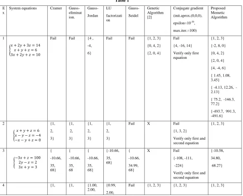
The proposed method is able to determine solutions of a system even if the number of equations is less than the number of unknowns, as can be seen in Example 7, Table 1. Also, the proposed method is able to determine solutions of a system even if the number of equations is larger than the number of unknowns, as can be seen in Example 8, Table 1. In Table 1 are listed experimental solutions obtained for several systems of equations, using some traditional methods and the method proposed in this paper.
It should be mentioned that the results posted inTable 1, last column, obtained with the proposed MA are not refined with traditional algorithms. For example, refining the solutions obtained with the proposed MA in Example 3, Table 1, using Gaussian elimination, leads to the solution{-10.668, 35.001, 68.000} which is much closer to the accurate solution.
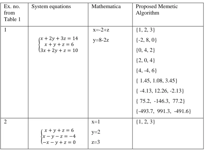
Remark: It should be noted that mathematical software such as Mathematica can produce a set of linearly independent vectors from which linear system solutions can be constructed. In Table 2 are given solutions obtained with Mathematica for some equations systems from Table 1. The values of the parameters used in the experiments are: - r =10;
- population size of each generation =1000 - maxim number of generations = 100
- maximum number of solutions inside an interval = 10 - maximum acceptable deviations aa=10
-10
It has been observed that the crossover technique does not help much, so the number of chromosomes generated by this technique was about 10% in a population.
As for mutations, it was observed that those that keep a part of the initial configuration of elites (mass-mutations) are the most productive.
[image:5.595.49.544.366.766.2]Also, we observed that if we use a more random population, the method performance increases.
Table 1
E x
System equations Cramer
Gauss-eliminat ion.
Gauss-
Jordan LU
factorizati on
Gauss-
Seidel
Genetic Algorithm [2]
Conjugate gradient
(init.aprox.(0,0,0),
epsilon=10-30,
max.iter.=100)
Proposed Memetic Algorithm
1
Fail Fail {4 ,
-4,
6}
Fail Fail {1, 2, 3}
{0, 4, 2}
{2, 0, 4}
Fail
{4, -16, 14}
Verify only first equation
{1, 2, 3}
{-2, 8, 0}
{0, 4, 2}
{2, 0, 4}
{4, -4, 6}
{ 1.45, 1.08, 3.45}
{ 4.13, 12.26, -2.13}
{ 75.2, -146.3, 77.2}
{-493.7, 991.3, -491.6}
2
{1,
2,
3}
{1,
2,
3}
{1,
2,
3}
{1,
2,
3}
Fail X Fail
{1, 3, 2}
Verify only first and second equation
{1, 2, 3}
3
{
-10.66,
35, 68}
{
-10.66,
35, 68
{
-10.66,
35, 68}
{-10.66,
35, 68}
{
-10.66,
34.99, 68}
X Fail
{-108, -111,
-224}
Verify only first and second equation
{-10.58,
34.80,
68.27}
4 {1, {1, {1.00,
2.00, {0.99,
2.00,
2,
3}
2,
3}
2.99} 3.00}
5
{0.5, 0.75,
1.0}
{0.5,
0.75,
1.0}
{0.50, 0.74,
0.99}
{0.5,
0.75,
1.0}
{0.50, 0.74, 0.99}
{0, 1, 1} Fail
{-6.5, 2.5, 8}
Verify only first and second equation
{0.55,
0.72,
0.97}
6
{3.16,
-2.3,
-1.5}
{3.16, -2.33,
-1.50}
{3.16, -2.33,
-1.50}
{3.16,
-2.33,
-1.50}
Fail X Fail
{1.05, 0.83, 0.61}
Verify only first equation
{3.16,
-2.33,
1.49}
7
Fail Fail Fail Fail Fail X Fail
{1, 1, 1}
{1.59,
0.80,
3.20}
8
Fail Fail {1,1} Fail Fail X Fail
{2, 0, 0}
Verify only first equation
{1,1}
9
{1,
1,
1}
{1,
1,
1}
{1, 0.99, 1}
{1,
0.99,
1}
{0.99,
1,
0.99}
{1, 1, 1} {0.97,
1.08,
1.19}
{1, 1, 1}
1 0
{1,
1,
1}
{1,
1,
1}
{0.99, 1,
1}
Fail Fail {1, 1, 1} Fail
{1.40, 0.79, 1}
Verify only first and second equation
{1, 1, 1}
1 1
{4,
5,
2}
{4,
5,
2}
{4, 4.99, 2}
{4,
5,
2}
Fail {4, 5, 2} Fail
{13, -8.5, 6.5}
Verify only first and second equation
{4, 5, 2}
[image:6.595.134.463.519.760.2]X: results are not available for this case.
Table 2
Ex. no. from Table 1
System equations Mathematica Proposed Memetic Algorithm
1
x=-2+z y=8-2z
{1, 2, 3} {-2, 8, 0} {0, 4, 2} {2, 0, 4} {4, -4, 6} { 1.45, 1.08, 3.45} { -4.13, 12.26, -2.13} { 75.2, -146.3, 77.2} {-493.7, 991.3, -491.6}
2
x=1 y=2 z=3
3
x=-10.66, y=35.00 z=68.00
{-10.58, 34.80, 68.27}
7
x=2.66-0.33z y=-1.33+0.66z
{1.59, 0.80, 3.20}
4.
CONCLUSION AND FUTURE WORK
It is concluded that MAs can be very helpful in finding solution for linear system of equations. Proposed MA worked accurate and were able to find solutions of the given linear system of equations, even in cases where traditional methods fail (determinant null, ill-conditioned systems, subdeterminate systems, supradeterminate systems, system doesn’t satisfy the convergence conditions, convergence condition satisfied but an infinite number of solutions found/not found, etc). By this it can be concluded that the proposed MA is more effective than traditional numerical methods for solving linear systems of equations.
In cases where no accurate solution for a linear system of equations can not be determined, an approximate solution is good and it can be obtained by the proposed method. The proposed algorithm is able to discover solutions whose fitness is very close to 0, which are good/acceptable in industrial applications.
There are situations when a linear system of equations has infinite solutions. In the present approach, the proposed method is able to find all the solutions inside of a given interval.
To discover more than one solution was used an incremental search of initial interval. In present approach, the size of incremental interval r is set by the user. A further concern will be a dynamical size adjustment of the r value, and even more, the determination of specific intervals and specific size of incremental interval r, different for each unknown in part. The proposed method is relatively simple to implement, but it still requires some further implementation refinements. This is in particular for cases where the solutions obtained by the proposed method, "oscillates" around the accurate solution, but do not "catch" the accurate solution, as in the examples 3,5 and 6 , Table 1. While running proposed MA for the presented problems, it was observed that even if MA is able to search for all the system’s solutions in a given interval [-r, +r], in some cases, the MA accuracy is lower than the accuracy of solutions found by iterative methods. A solution is to use the proposed MA combined with traditional methods (gaussian, LU, GJ etc) for refining the solutions. That's because present approach is based on discrete optimization [8]. In this case, the solutions are characterized by their fitness values and can be accurate or in the vicinity of optimum. As a future direction of study, an approach to the problem as an continuous optimization [8] problem is recommended. The MA schema developed above can also be implemented on parallel machines by allotting different equations to different machines in local search phase and this will be our preoccupation in the future.
5. REFERENCES
[1] Al Dahoud Ali , Ibrahiem M. M. El Emary, and Mona M. Abd El-Kareem, Application of Genetic Algorithm in Solving Linear Equation Systems, MASAUM Journal of Basic and Applied Science, Vol.1, No.2 Sept. 2009 [2] Ikotun Abiodun M., Lawal Olawale N.,Adelokun
Adebowale P. The Effectiveness of Genetic Algorithm in Solving Simultaneous Equations, International Journal of Computer Applications (0975 – 8887) Volume 14– No.8, February 2011
[3] Crina Grosan, Ajith Abraham, Multiple Solutions for a System of Nonlinear Equations, International Journal of Innovative Computing, Information and Control ICIC International , 2008 ISSN 1349-4198
[4] Ibrahiem M.M. El-Emary,Mona M. Abd El-Kareem, Towards Using Genetic Algorithm for Solving Nonlinear Equation Systems, World Applied Sciences Journal 5 (3): pp. 282-289, 2008, ISSN 1818-4952
[5] Crina Grosan, Ajith Abraham, A New Approach for Solving Nonlinear Equations Systems, IEEE Transaction on Systems, Man and Cybernetics-part A: Systems and Humans, vol. 38, no. 3, May 2008
[6] Yong Zhou, Huajuan Huang, Junli Zhang, Hybrid Artificial Fish Swarm algorithm for Solving Ill-Conditioned Linear Systems of Equations, ICICIS 2011 Proceedings, Part 1, Springer 2011, pp. 656-662 [7] Nikos E. Mastorakis, Solving Non-linear Equations via
Genetic Algorithms, Proceedings of the 6th WSEAS Int. Conf. on Evolutionary Computing, Lisbon, Portugal, June 16-18, 2005 pp24-28
[8] Ferrante Neri, Carlos Cotta, and Pablo Moscato (Eds.), Handbook of Memetic Algorithms, Studies in Computational Intelligence, 2012 Springer-Verlag Berlin Heidelberg, ISBN 978-3-642-23246-6
[9] Jason Brownlee, Clever Algorithms: Nature-Inspired Programming Recipes, 2011, ISBN:978-1-4467-8506-5 [10] Michel Gendreanu, J.Y.Potvin, Handbook of
Metaheuristics, Springer 2010, ISBN 978-1-4419-1663-1 [11] Teofilo F. Gonzales, Handbook of Approximation Algorithms and Metaheuristics, Chapman&Hall/CRC 2007