Size Biased Lindley Distribution and Its Properties a Special Case of Weighted Distribution

http://www.scirp.org/journal/am ISSN Online: 2152-7393

ISSN Print: 2152-7385

Size Biased Lindley Distribution and Its

Properties a Special Case of Weighted

Distribution

Arooj Ayesha

University of Agriculture, Faisalabad, Pakistan

Abstract

The purpose of this paper is to introduce a size biased Lindley distribution which is a special case of weighted distributions. Weighted distributions have practical significance where some types of biased occur in a density function,

i.e. probability is proportional to the size of the variate, that’s why the pro-posed version of size biased Lindley is designed for such situations more rea-sonably and more precisely. Principle properties of the density function are also discussed in this paper such as moments, measure of skewness, kurtosis, moment generating function, characteristics generating function, coefficient of variation, survival function and hazard function which are derived for un-derstanding the structure of the proposed distribution more briefly.

Keywords

Lindley Distribution, Weighted Distribution, Size Biased, Survival Function, Hazard Function

1. Introduction

Weighted Distributions

Weighted distributions are required when the recorded observation from an event cannot randomly sample from actual distribution. This happens when the original observation damaged as well as an event occur in non-observability manner. Due to these inappropriate situations, resulting values are reduced, and units or events do not have same chances of occurrences as if they follow the ex-act distribution.

Let the original observation x has pdf f x

( )

then in case of any biased in sampling appropriate weighted function, say w x

( )

which is a function of

ran-dom variable will be introduced to model the situation. How to cite this paper: Ayesha, A. (2017)

Size Biased Lindley Distribution and Its Properties a Special Case of Weighted Dis-tribution. Applied Mathematics, 8, 808-819.

https://doi.org/10.4236/am.2017.86063

Received: April 2, 2017 Accepted: June 16, 2017 Published: June 19, 2017

Copyright © 2017 by author and Scientific Research Publishing Inc. This work is licensed under the Creative Commons Attribution International License (CC BY 4.0).

http://creativecommons.org/licenses/by/4.0/

Then new density function w

( )

f x will be given by Equation (1), where _fw

represent a weighted distribution where w is considered as weighted function

( )

( ) ( )

w

f x =w x f x w (1) where w x

( )

is considered as normalizing factor which is utilized to create total

probability or area under the curve, equal to 1. If w x

( )

is constant term, then

( )

( )

w

f x = f x .

The Lindley distribution introduced with two parameters by Shanker et al. (2013) [1] by taking into account the survival and waiting time data. In Lindley exponential distribution Bhatti and Malik (2014) [2] studied its mathematical properties and checked its flexibility by using real data set. Due to one parameter of Lindley distribution, Zakerzadeh and Dolati (2009) [3] stated that it does not support for the better analysis of life time data they provide family of distribu-tion with three parameters which is more flexible for modeling of life time data. The geometric Lindley was extended by Mervociand Elbatal (2013) [4] into a new model called transmuted geometric Lindley. Lindley distribution and expo-nential distribution was compared by Ghitany et al. (2008) [5] in which it is con-cluded that model provide effective conclusion and they also check the flexibility of their properties. Poisson Lindley distribution was enlarged by Borah and De-ka Nath (2001) [6] with further study called inflated Poisson Lindley distribu-tion. Ghitany et al. (2007) [7] came up with a comparison of two models and showed that Lindley distribution provide effective model than exponential dis-tribution. Whereas Ghitany et al. (2008) [8] examined the Poisson Lindley dis-tribution to model count data, as well as Ghitany et al. (2008) [9] aims their study for data does not include zero counts, since Zakerzadeh and Dolati (2009)

[10] described generalized form of Lindley distribution with three parameters. Therefore Ghitany et al. (2011) worked on modeling of survival data and intro-duced a Lindley distribution with two parameters called weighted Lindley dis-tribution although Lord and Geedipally (2011) [11] proposed a new distribution called negative binomial Lindley, contains two parameter for crash count data. Mazcheli and Achcar (2011) [12] worked on competing risk data. Bakouch et al.

(2012) [13] proposed extended form of Lindley distribution to model the life time data to check its reliability, failure rate function. Whereas Elbatal et al.

(2013) [14] proposed that Lindley distribution is a mixture of both gamma and exponential distribution. Shanker et al. (2013) [15] compared one parameter Lindley distribution with two parameter Lindley distribution. While Wang (2013) [16] introduced a life time distribution with three parameters, although Bhati and Malik (2014) [17] worked at Lindley random variable and bring in to being a new family of distribution for remission times uncensored data of 128 cancer bladder patients. Mervoci and Sharma (2014) [18] extended the Lindley distribution called beta Lindley distribution. Whereas Singh et al. (2014) gave truncated Lindley distribution.

2. Methodology

f(x) and normalizing factor is E(x) to make total area is to be 1. Mathematically,

( )

xf x

_{( )}

( )

g x

E x =

Some structural properties discussed by using simple algebraic methods whe-reas some results of primary and size biased density function are compared based on random samples for each density function. For data simulation and calculation of results based on these samples r programming language is used. Both functions are compared based on these results of simulation, for different values of parameter

θ

.

1) One parameter Lindley distribution

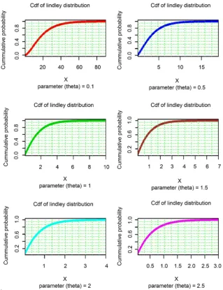
A one parameter Lindley distribution with parameter θ is defined by its prob-ability density function given as.

( )

; 2

(

1

)

e , 0 1

x

x

f x x

θ θ θ θ − + = >

+ (2)

Plot of probability function of Lindley distribution (see Figure 1 and Table 1) 2) Raw moments

The th

r moments about origin of one parameter Lindley distribution is given by Equation (3)

(

)

(

)

! 1

, 1, 2, 3, 1 r r r r r µ θ θ θ + + = = +

′ _ (3)

Taking r=1, 2, 3 and 4 in this equation the first four moments about origin

is obtained as

(

)

1 2 1 θ µ θ θ + ′ = + 2 2 2 3 1 θ µ θ θ +   = _{ } +   ′ 3 2 6 4 1 θ µ θ θ +   = _{ } +   ′

(

)

(

)

4 4 24 5 5 µ θ θ θ + ′ = +

3) Moments about mean of one parameter Lindley distribution Then central moments are obtained as,

(

)

1 2 1 θ θ µ θ + = +

(

)

(

)

2

2 2 2

4 2 1

θ

θ

µ

θ

θ

+ + = +

(

)

(

)

3 2

3 3 3

2 6 6 2

1

θ

θ

θ

µ

θ θ

+ + +

=

[image:4.595.206.536.72.496.2]

Figure 1. Graphical behavior of Lindley distribution for some values of parameter θ.

Table 1. Central moments and standard deviation for different values of parameter θ.

Lindley

distribution μ1 μ2 μ3 μ4 Std. Dev

θ = 0.1 19.09091 199.1736 3998.497 239006.2 14.11289

θ = 0.5 3.333333 7.555556 31.40741 362.0741 2.748737

θ = 0.9 1.695906 2.192127 5.195381 32.24576 1.480583

θ = 1.3 1.103679 0.994396 1.656285 6.953597 0.9971941

[image:4.595.208.539.543.732.2]

(

)

(

)

4 3 2

4 4 4

3 3 24 44 32 8 1

θ

θ

θ

θ

θ

µ

θ

+ + + +

=

+

4) Cumulative distribution function of Lindley distribution Cdf of the Lindley distribution is given by Equation (4)

( )

₀x

( ) ( )

d

F x =

∫

f x x

(

)

_{( )}

2 0

1 e

d 1

x

x x

x

θ

θ θ

−

+ +

∫

This gives,

( )

1 e 1

1

x x

F x θ θ

θ

−  

= − _ + _

+

  (4)

[image:5.595.214.534.298.714.2]

Plot of cumulative distribution function of Lindley distribution (see Figure 2) 5) Moment generating function of Lindley distribution

( )

₍

(

₎₍

₎

)

2 2 1 1 x t t M t θ θ θ θ − + = + +

6) Characteristic generating function of Lindley distribution

( )

(

₍

₎

)

2 2 1 1 x it it M it

θ

θ

θ

θ

− + = + −

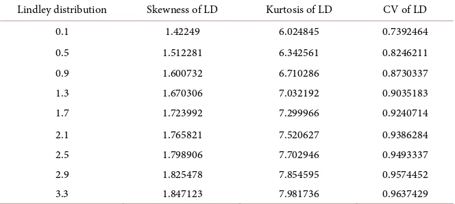
[image:6.595.207.539.583.732.2]

7) Skewness, Kurtosis and Coefficient of variation of Lindley distribution (see

Table 2)

(

)

(

)

3 2

3 2 2

2 6 6 2

Skewness

4 2

θ θ θ

θ θ + + + = + +

(

)

(

)

4 3 2

2 2

3 3 24 44 32 8 Kurtosis

4 2

θ θ θ θ

θ θ + + + + = + + 2 4 2 C.V 2 θ θ θ + + = +

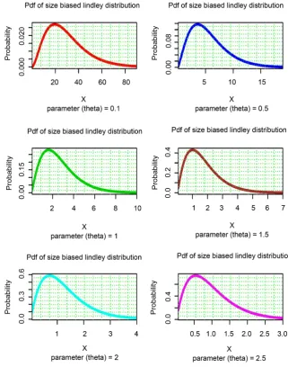
8) Size biased Lindley distribution

The probability density function of size biased Lindley distribution is given as

(

)

( )

(

_{( )}

,

)

,

x xf x

f x g x

E x

θ

θ = =

( )

3

(

1

)

e

; , 0

2

x

x x

g x x

θ θ θ θ − +

⇒ = >

+ (5)

Plot of probability function of size biased Lindley distribution (see Figure 3) 9) Raw moments of size biased Lindley distribution

(

) (

)

2

2 1 ! 2

r

r r r

µ θ θ

θ +

= + + +

′ _ _{ (6)}

Taking r=1, 2, 3 and 4 in this equation the first four moments about origin

is obtained as

(

)

(

)

1 2 3 2 θ µ θ θ + ′ = +

Table 2. Skewness, kurtosis and coefficient of variation for some values of parameter θ.

Lindley distribution Skewness of LD Kurtosis of LD CV of LD

0.1 1.42249 6.024845 0.7392464

0.5 1.512281 6.342561 0.8246211

0.9 1.600732 6.710286 0.8730337

1.3 1.670306 7.032192 0.9035183

1.7 1.723992 7.299966 0.9240714

2.1 1.765821 7.520627 0.9386284

2.5 1.798906 7.702946 0.9493337

2.9 1.825478 7.854595 0.9574452

[image:7.595.207.529.75.484.2] [image:7.595.339.405.519.618.2]

Figure 3. Graphical behavior size biased density function for some values of parameter.

(

)

(

)

2 2

6 4

2

µ θ

θ θ

+ ′ =

+

(

)

(

)

3 3

24 5 2

µ θ

θ θ

+ ′ =

+

(

)

(

)

4 4

120 6 2 θ µ

θ θ

+ ′ =

+

10) Moments about mean of size biased Lindley distribution (see Table 3) Central moments of size biased Lindley distribution are obtained as:

(

)

(

)

1

2 3

2 θ θ µ

θ

+ =

+

(

)

(

)

2

2 2 2

2 6 6

2

θ

θ

θ θ

µ

= + +

[image:8.595.206.539.90.254.2]

Table 3. Central moments and standard deviation for different values of parameter θ.

SBLD μ1 μ2 μ3 μ4 Std. Dev

θ = 0.1 29.52381 299.7732 5999.784 449591.7 17.31396

θ = 0.5 5.6 11.84 47.872 708.4032 3.44093

θ = 0.9 2.988506 3.584798 8.148448 65.90233 1.297429

θ = 1.3 2.004662 1.683321 2.675344 14.75241 1.297429

θ = 1.7 1.494436 0.9650163 1.181765 4.916901 0.9823524

θ = 2.1 1.184669 0.6207837 0.6188595 1.025826 0.7878983

θ = 2.5 0.9777778 0.4306173 0.3620521 1.002462 0.6562144 θ = 2.9 0.8304011 0.3150689 0.2290128 0.5418929 0.56131 θ = 3.3 0.7204117 0.2398822 0.1535249 0.3168071 0.4897777

(

)

(

)

3 2

3 3 3

4 9 180 12

2

θ

θ

θ

θ θ

µ

= + + +

+

(

)

(

)

4 3 2

4 4 4

24 12 42 60 30

2

θ

θ

θ

θ

θ θ

µ

= + + + +

+

11) Cumulative distribution function of size biased Lindley distribution Cdf of size biased Lindley distribution is given by,

( )

₀x

( ) ( )

d

G x =

∫

g x x

( )

₀ 3

(

1

)

e d

( )

2

x

x x x

G x x

θ θ θ − + = +

∫

( )

3 ₀

(

1

)

e d

( )

2

x _x

G x θ x x θ x

θ −

= +

+

∫

This gives

( )

2 2e

(

2

)

(

1 e

(

1

)

)

2

x x

x x

G x

θ _{θ θ} θ _θ

θ

− −

− − + + − +

=

+ (7)

Please see Figure 4:

12) Moment generating function of size biased Lindley distribution

(

)

(

)

(

)

3 3 2 M.G.F 2 t t θ θ θ θ − + − = − +

13) Characteristics generating function of size biased Lindley distribution

(

)

(

)

(

)

3 3 2 C.F 2 it it θ θ θ θ − + − = − +

14) Skewness, Kurtosis and Coefficient of variation of size biased Lindley dis-tribution (see Table 4).

(

)

(

)

{

}

3 2 1 3 2 2

4 9 18 12

Skewness

2 6 6

θ θ θ

β

θ θ

+ + +

= =

[image:9.595.210.523.75.459.2]

Figure 4. Graphical behavior of cumulative density function of size biased Lindley dis-tribution for some values of parameter.

Table 4. Skewnesskurtosis and coefficient of variation of SBLD for some values of

para-meter.

θ Skewness SBLD Kurtosis of SBLD CV of SBLD

0.1 1.155969 5.003023 0.5864406

0.5 1.175044 5.053324 0.6144518

0.9 1.200544 5.128277 0.6335461

1.3 1.224981 5.206302 0.6472056

1.7 1.246606 5.279858 0.6573401

2.1 1.265265 5.34658 0.6650788

2.5 1.28125 5.406111 0.6711283

2.9 1.294946 5.458867 0.6759504

3.3 1.306718 5.505525 0.6798582

(

)

(

)

{

}

4 3 2

2 2

2

24 12 42 60 30

Kurtosis

2 6 6

θ

θ

θ

θ

β

θ

θ

+ + + +

= =

[image:9.595.208.540.533.677.2]

(

)

(

)

1

2

2 6 6

C.V

2 3

θ δ

θ µ

θ

′

+ + = =

+

15) Survival function of size biased Lindley distribution

( )

e 2 2 2

2 2

2

t

S t t t t

θ

θ θ θ θ

θ

−

 

= _ + − + + _

+

16) Hazard function of size biased Lindley distribution

( )

32

(

)

2 2

1

2 2

t t

H t

t t t

θ

θ θ θ θ

+ =

[image:10.595.213.450.80.209.2] [image:10.595.208.539.305.504.2]

+ − + +

[image:10.595.208.539.537.734.2]

Table 5 and Table 6 show some results of original and size biased Lindley distribution respectively which are based on random samples that are generated for different values of the parameter θ. Each sample is based on 10,000 observa-tions.

Table 5. Results based on random samples from Lindley distribution.

LD Mean Variance _deviation Standard Median Skewness kurtosis

θ = 0.1 17.280 128.6998 11.34459 14.960 0.7519824 2.899294

θ = 0.5 3.221 7.572646 2.751844 2.485 2.485 6.332139

θ = 0.9 1.610 2.119268 1.455771 1.245 1.671199 7.427447 𝜃𝜃 = 1 1.403 1.582653 1.258035 1.042 1.62406 6.789065 θ = 1.3 1.054 0.979174 0.9895322 0.765 1.776654 7.588966 θ = 1.7 0.7706 0.5534715 0.7439567 0.5500 1.761394 4.358188 θ = 2.1 0.5875 0.3416315 0.5844925 0.4200 1.8265 7.129288 θ = 2.5 0.4656 0.2213501 0.4704785 0.3050 2.072667 9.192622 θ = 2.9 0.4014 0.1666295 0.4082028 0.2650 2.119914 9.657423 θ = 3.3 0.3386 0.1222347 0.3496208 0.2150 2.038068 8.910684

Table 6. Results based on random samples from size biased Lindley distribution.

SBLD Mean Variance Standard _deviation Median Skewness Kurtosis

θ = 0.1 24.570 132.92 11.5291 23.280 0.2377253 2.158117

θ = 0.5 5.615 12.35464 3.514917 4.925 1.158568 5.12711

θ = 0.9 2.950 3.502266 1.871434 2.550 1.278998 5.439581

θ = 1 2.647 2.879649 1.696953 2.310 1.265753 5.273339

By comparing the results in above tables, it is noted that mean, median, and standard deviation all these measures are greater in magnitude for size biased distribution as compared to actual distribution for respective values of parame-ter.

References

[1] Bhati, D., Malik, M.A. and Vaman, H.J. (2014) Lindley-Exponential Distribution: Properties and Applications.Metron, 73, 335-357.

[2] Borah, M. and Nathl, A.D. (2001) A Study on the Inflated Poisson Lindley Distribu-tion. Journal of the Indian Society of Agricultural Statistics, 54, 317-323.

[3] Das, K.K. and Roy, T.D. (2011) Applicability of Length Biased Weighted Genera-lized Rayleigh Distribution. Advances in Applied Science Research, 2, 320-327. [4] Elbatal, I., Merovci, F. and Elgarhy, M. (2013) A New Generalized Lindley

Distribu-tion. Mathematical Theory and Modeling, 3, 30-47.

[5] Ghitany, M.E. and Al-Mutairi, D.K. (2008) Size-Biased Poisson-Lindley Distribu-tion and Its ApplicaDistribu-tion. Metron-International Journal of Statistics, 66, 299-311. [6] Ghitany, M.E., Atieh, B. and Nadarajah, S. (2008) Lindley Distribution and Its

Ap-plication. Mathematics and Computers in Simulation, 78, 493-506.

https://doi.org/10.1016/j.matcom.2007.06.007

[7] Ghitany, M.E., Al-Mutairi, D.K. and Nadarajah, S. (2008) Zero-Truncated Poisson- Lindley Distribution and Its Application. Mathematics and Computers in Simula-tion, 79, 279-287. https://doi.org/10.1016/j.matcom.2007.11.021

[8] Ghitany, M.E., Alqallaf, F., Al-Mutairi, D.K. and Husain, H.A. (2011) A Two-Pa- rameter Weighted Lindley Distribution and Its Applications to Survival Data. Ma-thematics and Computers in Simulation, 81, 1190-1201.

https://doi.org/10.1016/j.matcom.2010.11.005

[9] Lord, D. and Geedipally, S.R. (2011) The Negative Binomial-Lindley Distribution as a Tool for Analyzing Crash Data Characterized by a Large Amount Of Zeros. Acci-dent Analysis & Prevention, 43, 1738-1742.

https://doi.org/10.1016/j.aap.2011.04.004

[10] Mazucheli, J. and Achcar, J.A. (2011) The Lindley Distribution Applied to Compet-ing Risks Lifetime Data. Computer Methods and Programs in Biomedicine, 104, 188-192. https://doi.org/10.1016/j.cmpb.2011.03.006

[11] Merovci, F. and Sharma, V.K. (2014) The Beta-Lindley Distribution: Properties and Applications. Journal of Applied Mathematics, 2014, Article ID: 198951.

https://doi.org/10.1155/2014/198951

[12] Mir, K.A. and Ahmad, M. (2009) Size-Biased Distributions and Their Applications.

Pakistan Journal of Statistics, 25, 283-294.

[13] Patil, G.P. and Rao, C.R. (1978) Weighted Distributions and Size-Biased Sampling with Applications to Wildlife Populations and Human Families. Biometrics, 34, 179-189. https://doi.org/10.2307/2530008

[14] Ratnaparkhi, M.V. and Naik-Nimbalkar, U.V. (2012) The Length-Biased Lognor-mal Distribution and Its Application in the Analysis of Data from Oil Field Explo-ration Studies. Journal of Modern Applied Statistical Methods, 11, 22.

[15] Shanker, R., Sharma, S. and Shanker, R. (2013) A Two-Parameter Lindley Distribu-tion for Modeling Waiting and Survival Times Data. Applied Mathematics, 4, 363- 368. https://doi.org/10.4236/am.2013.42056

Inference and Application. Journal of Statistics Applications & Probability, 3, 219- 228. https://doi.org/10.12785/jsap/030212

[17] Wang, M. (2013) A New Three-Parameter Lifetime Distribution and Associated In-ference. arXiv:1308.4128

[18] Zakerzadeh, H. and Dolati, A. (2009) Generalized Lindley Distribution. Journal of Mathematical Extension, 3, 13-25.

Submit or recommend next manuscript to SCIRP and we will provide best service for you:

Accepting pre-submission inquiries through Email, Facebook, LinkedIn, Twitter, etc. A wide selection of journals (inclusive of 9 subjects, more than 200 journals)

Providing 24-hour high-quality service User-friendly online submission system Fair and swift peer-review system

Efficient typesetting and proofreading procedure

Display of the result of downloads and visits, as well as the number of cited articles Maximum dissemination of your research work