Design and Implementation of jAHP: A Java-based
Analytic Hierarchy Process Application
Chen-Huei Chou
School of Business
College of Charleston
Charleston, SC, USA
ABSTRACT
Solving a multiple criteria decision making problem by a group of decision makers in different geographical locations could be hard. Analytic Hierarchy Process is a mathematical model capable of dealing with such type of problems. However, the lack of geographical support is the major drawback of a traditional standalone Analytic Hierarchy Process tool. To address this issue, this paper proposes to adopt Java programming language to design and implement jAHP, a Java-based Analytic Hierarchy Process application available over the Internet. External validity is accessed by comparing jAHP results with both manual approach and commercial software.
Keywords
Analytic Hierarchy Process (AHP), Java Programming, JTree
1.
INTRODUCTION
Decision making process can be finalized by an individual or a group of people. Decision-making problems usually consist of multiple decision-making criteria. In order to manage and evaluate the criteria systematically, a reliable and easy to use method is usually favorable. The Analytic Hierarchy Process (AHP) [8, 9, 13] is a mathematicalmodel capable to deal with multiple criteria decision-making problems. The potential drawback of a traditional desktop version of AHP tool is the lack of support when decision makers are in different geographical locations.
Java is a programming language used to create desktop applications running on top of Java Virtual Machine across different platforms such as Microsoft Windows, Mac OS, Linux, and so on. The Java desktop applications can also be converted to be executed over the Internet through Web browsers.
In order to overcome the decision makers’geographical issue, this paper proposes the use of Java programming language for the design and implementation of jAHP, a Java-based Analytic Hierarchy Process application.The jAHP can be used as a standalone as well as a Web-based decision-making tool. Specially, this paper attempts to answer the following questions:
Can Java program be used as a programming language for
designing and implementing Analytic Hierarchy Process?
How can one access the Analytic Hierarchy Process
application over the Internet?
How can one access external validity of the implemented
program?
The rest of the paper is organized as follows. The details of AHP and applications of AHP are discussed in section 2. The design and implementation of jAHP are descripted in section 3. External validity is accessed in section 4 by comparing jAHP results with both manual approach and commercial software.
2.
BACKGROUND
2.1
Analytic Hierarchy Process
The Analytic Hierarchy Process is a method useful for dealing with multiple criteria decision-making problems.While it is suitable for both individual and group decision-making circumstances, it is more often used in a group setting.The goal of AHP is to compute an overall score by aggregating weights from various decision elements.Also, alternatives of decisions are ranked, and the one with the highest score is the final decision.Using AHP, a decision-making problem is broken down into criteria and sub-criteria in a hierarchy of interrelated decision elements.Sub-criteria under a decision element are the details of that criterion.The top level of a multi-level AHP structure is the goal of the decision-making problem, while the lowest level consists of the alternatives of decisions.
Figure 1 presents a typical form of a decision-making model in the Analytic Hierarchy Process.It consists of k levels; level 1 is the goal of the problem and level k includes all alternatives of decision. The levels between these two levels are criteria structured from the top to the bottom in a general to specific fashion.
The goal of the decision-making
problem
Criterion 1 Criterion 2 Criterion 3 Criterion n
Sub-Criterion 1
Sub-Criterion 2
Sub-Criterion i Sub-Criterion
3
...
...
Level 1
Level 2
Level 3
Level k
...
Decision Alternative 1
Decision Alternative 2
Decision Alternative 3
Decision Alternative m
...
[image:1.595.321.542.544.692.2]In addition, a four-step process is applied when using AHP to solve a decision-making problem.It consists of the following steps:
Step 1: Formulation of the decision hierarchy. Step 2: Evaluation of the decision elements.
Step 3: Calculation of the relative weights of decision elements.
Step 4: Generation of a set of ratings for the decision alternatives by aggregation of relative weights.
The main purpose of Step 1 is to identify decision elements in a hierarchical manner.First, the goal of the decision is set as the root node of the structure.The main criteria of the decision are then identified and listed in the next level (level 2) to the goal.The sub-criteria of the criteria identified are also listed in the next level of the corresponding criterion.The same process is repeated until there is no sub-criterion to be identified.Finally, the decision elements in a hierarchical structure are constructed.
Step 2 deals with the evaluation of decision elements identified in Step 1.There are two main approaches for evaluation of decision elements: pairwise comparison and direct assignment.The pairwise comparison approach applies consistent comparison to multiple items, thus dealing with the difficulty the human brain faces when comparing multiple items.In using pairwise comparison, two elements are compared each time.If there are N elements to be compared, the total amount of pairwise comparisons is .However, the pairwise comparison approach may not be able to efficiently handle the huge size of elements being pairwisely compared.The main drawback of pairwise comparison is that the amount of comparison increases exponentially when the total number of elements increases.Also, it is more likely to have incomplete ratings from experts when the size of elements being evaluated is too large.
To address this drawback, direct assignment is used to reduce the amount of comparisons.In this approach, decision makers assign the relative importance of elements directly for each element.However, the major challenge of this approach is the reliability and consistency of results, compared to the pairwise comparison approach.Ramadhan et al. [7] conducted an empirical study using AHP to rank the priority of pavement maintenance, which includes large number of decision elements.They found that the results generated by pairwise comparison and by direct assignment were statistically similar.It is safe to use the direct assignment approach with reliability and consistency when a huge number of decision elements is involved.Thus, direct assignment is the best option when too many elements are being compared or the size of total comparison is too large.
Therefore, the method for the evaluation of decision elements by these two approaches is also different.When the pairwise comparison approach is applied, the values of relative importance between each pair of two elements are stored in a comparison matrix A, where the relative importance is in a scale of 1 to 9 (see Table 1).The size of the matrix is n×n if n elements in total are compared.The diagonal values in the matrix are unity, that is aii=1.Cells in the upper diagonal and
cells in the lower diagonal are in reciprocal relationship, that is
where j>i.Thus, only half of the elements, usually in
upper diagonal, in the matrix are collected by airwise comparisons, excluding diagonal ones.The comparison is then normalized through dividing each element by the sum of elements in its column [10].The cells in the normalized
comparison matrix Anormalized are
for j=1, 2,
…,n.As a result, priority vector is a 1×n matrix containing the weights, where
[image:2.595.315.544.176.446.2]for i=1, 2, …,n.When the direct assignment approach is applied, a decision maker rates the relative importance of elements directly.Therefore, the priority vector contains the weights that are normalized by the values of elements in the same group.
Table 1. Scale of relative importance [9, p. 843]
Intensity of Relative Importance
Definition Explanation
1 Equal
importance
Two activities contribute equally to the objective. 3 Moderate
importance of one over another
Experience and judgment slightly favor one activity over another
5 Essential or strong importance
Experience and judgment strongly favor one activity over another.
7 Demonstrated importance
An activity is strongly favored and its dominance is demonstrated in practice.
9 Extreme
importance
The evidence favoring one activity over another is of the highest possible order of affirmation.
2, 4, 6, 8 Intermediate values between the two adjacent judgments
When compromise is needed.
Step 3 calculates the relative weights of decision elements, which are the weights in the priority vector discussed above.If there is only one decision maker for evaluation, the relative weights are the values stored in the priority vector.However, usually several decision makers are involved in the evaluation of relative importance of elements.In this case, the relative weights are calculated by synthesizing the evaluations by multiple raters using geometric mean [1].
Step 4 generates a set of ratings on alternatives by aggregating relative weights (priority vectors in Step 3).This set of ratings toward the goal is represented by a vector of composite weights.The composite weights can be aggregated by either the distributed mode or the ideal mode [10].In the distributed mode, all alternatives are considered and the sum of composite weights from all alternatives is one.In the ideal mode, the best alternative is derived without the consideration of other alternatives.Through the aggregation process, relative weights for each decision element are divided by the maximum relative weight of that element.That is, the relative weight of the best alternative is one.
There are two types of priority values: local priority and global priority [10].The local priority is the weight in the priority vector of an element (discussed in Step 3).The global priority is the multiplication of the local priority of the element to the global priority of the parent element:
, where LPi is the local priority of element in level i
Also, the sum of the global priority to the elements in the lowest level (leaves) is one:
, where n is the number of nodes in the lowest
level and GPi is the global priority of ith element of these
nodes.
As a result, composite weights of an alternative can be aggregated by the global priority of all nodes in the lowest level:
, where GPi is the global priority of ith
element in the lowest level, Evali is the evaluation of
alternative to the ith element, and n is the number of nodes in the lowest level.
2.2
Applications of AHP
AHP is originally proposed to solve complex decision-making problems and has been successfully applied to diverse and numerous applications.Based on the review of applications by Zahedi[13], AHP had been applied to the following applications: economics and planning; energy (policies and allocations of resources); health; conflict resolution, arms control, and world influence; material handling and purchasing; flexible manufacturing systems; manpower selection and performance measurement; project selection; marketing; database management system selection; microcomputer selection; budget allocation; portfolio selection; model selection for cost-volume-profit analysis; accounting and auditing; education; politics; subjective probability estimation and cross impact analysis; sociology; interregional migration patterns; behavior under competition; environment; architecture; measuring the membership grade in fuzzy sets; methodology development; consulting.Moreover, Vaidyaa and Kumar [12] classified the applications of AHP into 10 fields: selection; evaluation; benefit-cost analysis; allocations; planning and development; priority and ranking; decision making; forecasting; medicine and related fields; AHP as applied with quality function deployment.
Several prior studies utilized AHP as an application of ranking for different purposes.For example, [2] applied it to locate and rank suitable sites for waste water treatment (soil aquifer treatment).[3] used it to rank enterprises based on their business efficiency.[11] predicted the ranking of soccer teams based on six criteria.
3.
JAVA IMPLEMENTATION OF JAHP
Following design science approach [4, 6], the application is implemented using the Java programming language and running on top of Java Virtual Machine. The application is encapsulated in the format of an executable jar.
3.1
Mapping AHP Hierarchy to Java
The major task of jAHP is the formation of decision hierarchy in Java. Other mathematical computations in AHP can be easily handled by most of programming languages. Java is an object-oriented language. Through inheritance, objects created could form tree-like hierarchical relationships. However, such relationships could not be mapped to AHP analogicallydue to the lack of a proper holding structure for the objects.
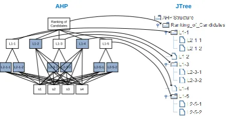
JTree, a class in Java[5], allows creating a structure withhierarchical nodes. Such tree-like structure is analogical to AHP structure with hierarchical decision criteria.Therefore, jAHP is designed to adopt such analogy between AHP and JTree.All nodes from AHP are mapped to JTreeone by one from the root to the leaves, in a breadth first manner. Figure 2
shows the mapping from AHP to JTree. Initially, JTree is empty and includes a document node called AHP Structure. Following the breadth first traversal in AHP structure, the root of AHP—Ranking of Candidates—ismapped to the root of JTree. Next, each corresponding node in AHP is added to the JTreelevel by level. By clicking “Add Node” button in jAHP, a node, mapped from AHP, can be added to JTree. A node can also be deleted by clicking “Remove Node” button (see a screenshot of jAHP in Figure 4 used for latter discussion).
Ranking of Candidates
L1-3 L1-2
L1-1 L1-4 L1-5
L2-1-1 L2-1-2 L2-3-1L2-3-2 L2-5-1L2-5-2
s2 s3
s1 s4
[image:3.595.316.538.185.301.2]AHP JTree
Fig. 2: Mapping AHP to JTree
The tree structure in jAHP, maintained by the mapping of AHPstructure to JTree, can be virtually traversed by the application or manually browsed by users.When traversed by the application, priority vectors are prepared. The tree structure in jAHP is able to be expanded and collapsed while browsing the structure by users.For the ease for navigation, expand all and collapse all to expand all nodes for details or collapse all nodes to show only the top level elements are implemented.These two functionalities are available as a pop-up window by right-clicking on top of the tree structure sub-window.
3.2
Relative Importance of Decision
Elements and Priority Vectors in jAHP
In jAHP, each node in JTree carries its own variables for computing AHP composite weights. Based on decision maker’s opinion, relative importance of each node is stored in jAHP by clicking “Relative Importance” for each selected node. Once the ratings of relative importance for a group of siblings are ready, normalization is applied. While computing weights, local priority and global priority of each node are updated.
3.3
Evaluation of Alternatives in jAHP
3.4
Web-based jAHP
Making the jAHP application accessible over Internet would address the issue of decision makers located in different places. In order to access the jAHP through the Web, the program is implemented through JApplet class. In addition, <applet> tags are added to the webpage loading the Web-based jAHP. The tags to be added is similar to the following:
<applet code= "jAHP.class"
width= "1000"
height= "700">
</applet>
4.
VALIDATION OF JAHP
In order to access external validityof the implementedjAHP, the results created by a running example are compared with both manual approach and commercialAHP software. First, a running example is presented in section 4.1. The results using implementedjAHP are included in section 4.2. Section 4.3 presents the progress in detail by manual approach.Finally, section 4.4 shows the results generated from commercial software Expert ChoiseTM.
4.1
Running Example
The running example shared in this section is a make-up decision making three-levelAHP hierarchicalstructure listed in Figure 3. Since the alternatives (candidates) are compared toward the leaves of the AHP structure, a complete AHP structure with all leaves in the same level may not reflect potential errors of the implementation of jAHP. Thus, an incomplete AHP structure is used. In this example, the goal (level 1) is the ranking of four candidates in terms of their completeness of decision elements. There are five main criteria (L1-1, L1-2, L1-3, L1-4, and L1-5) in level 2 and a total of six sub-criteria in level 3 (1-1, 1-2, 3-1, L2-3-2, L2-5-1, and L2-5-2). Among the six criteria in the level 3, L2-1-1 and L2-1-2 are the sub-criteria of L1-1; L2-3-1 and L2-3-2 are the details of L1-3; L2-5-1 and L2-5-2 are the sub-criteria of L1-5. In the last level, s1, s2, s3, and s4 represent alternatives (candidates). In order to save space formanual validation, direct assignment approach, rather than pair-wise comparisons approach,is used. Using direct assignment, the relative importance for the elements L1-1, L1-2, L1-3, L1-4, L1-5 in level 2 is assigned as 7.2, 8, 9.3, 6.5, and 2.2, respectively.Similarly, the relative importance of the elements in level 3 is assigned by 7.5, 7.1, 9.2, 9.1, 1.2, and 3.3, respectively for L2-1-1, L2-1-2, L2-3-1, L2-3-2, L2-5-1, and L2-5-2.
Ranking of Candidates
L1-3 L1-2
L1-1 L1-4 L1-5
L2-1-1 L2-1-2 L2-3-1 L2-3-2 L2-5-1 L2-5-2
s2
Level 1
Level 2
Level 3
[image:4.595.314.545.167.278.2]Alternatives s1 s3 s4
Fig.3: AHP structure of the running example
Moreover, Table 2 shows the evaluation of alternatives toward decision criteria. “P” indicates a presence of a criterion in the alternative and “A” indicates an absence of a criterion in the alternative. For example, when evaluating alternatives toward a decision criterion L1-1, s1 and s4 carry this decision criterion while s2 and s3 do not.
Table 2.Evaluation of alternatives toward decision criteria
Altern
ati
v
e
L1
-1
L1
-2
L1
-3
L1
-4
L1
-5
L2
-1
-1
L2
-1
-2
L2
-3
-1
L2
-3
-2
L2
-5
-1
L2
-5
-2
s1 P P P P A P P P P A A
s2 P P A P A P A A A A A
s3 A A P P P A A A P A P
s4 P P P P P A A P A P P
4.2
Results of jAHP
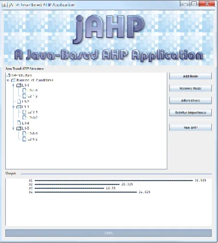
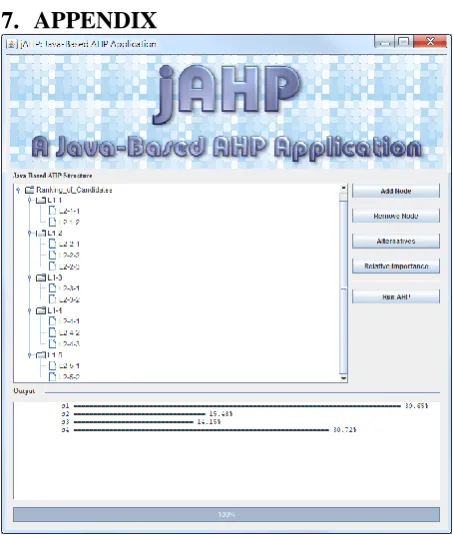
[image:4.595.316.542.456.707.2]Figure 4 shows the screenshot of the jAHP.The main sub-window located in the center left is the area to display the AHP structure, stored in JTree.The buttons located in the center right provide functionalities for different purposes.The sub-window in the bottom area is the output window for displaying final AHP composite weights.The very bottom part of the program is a progress bar indicating the percentage of work done. Using the mapped structure in the running example and setting the relative importance of elements and evaluations of alternative toward decision criteria with the same values, the final AHP composite weights is displayed in the output window. The composite weights for (s1, s2, s3, s4) are (38.56%, 20.32%, 16.50%, 24.52%).
[image:4.595.61.277.602.728.2]4.3
Manual Validation
The manual validation is to follow the four-step AHP computation discussed in section 2.1. After completing step 1, the AHP structure is constructed in the running example (section 4.1). Using direct assignment approach, the relative importance of element in the hierarchical structure are assigned (step 2). The first two steps are common to the manual validation, jAHP, and validation with Expert Choice.
Step 3 of AHP process is to prepare priority vectors. After normalization by dividing each value by the sum of them in level 2, the normalized relative importance for each of them is 0.2169, 0.2410, 0.2801, 0.1958, and 0.0663. These are the local priority values of these elements. Similarly,with the normalization process applied in the three groups located in level 3, the normalized relative importance becomes 0.5137, 0.4863, 0.5027, 0.4973, 0.2667, and 0.7333. The sum of the normalized relative importance for each group is one. These are also the local priority values of these six elements in the third level.Table 2 lists all values of local priority in the second column for the elements in level 2 and in the fifth column for the elements in level 3.
Step 4 is to generate a set of ratings for the decision alternatives by aggregation of relative weights. First, global priority for each node is calculated by , where LPi is
the local priority of element in level i along the path from the root to the element in level k. Therefore, the global priority for the elements in level 2 is the same as the local priority to that element (see the third column). Following the formula, the global priority for the elements in level 3 is the multiplication of the local priority to the element (in level 3) and the local priority to the parent element (in level 2). The results are listed in the 6th column of Table 3. For example, global priority of L2-1-1 is the products of local priority of L2-1-1 and local priority of L1-1. That is, GP(L2-1-1)=LP(L2-1-1)×LP(L1-1)=0.5137×0.2169=0.1114. Similarly, the global priority to other elements in level 3 can be calculated in the same way. Also, the sum of global priority to the elements in the lowest level (shaded ones in Figure 4) is one.That is, GP(L1-2)+GP(L1-4)+GP(L2-1-1)+GP(L2-1-2)+GP(L2-3-1)+GP(L2-3-2)+GP(L2-5-1)+GP(L2-5-2)=1.
Table 3. Local priority and global priority of each criterion in level 2 and level 3
Level 2 Level 3
Criteria Local
Priority Global Priority Sub-Criteria Local Priority Global Priority
L1-1 0.2169 0.2169 L2-1-1 0.5137 0.1114 L2-1-2 0.4863 0.1055
L1-2 0.2410 0.2410 – – –
L1-3 0.2801 0.2801 L2-3-1 0.5027 0.1408 L2-3-2 0.4973 0.1393
L1-4 0.1958 0.1958 – – –
L1-5 0.0663 0.0663 L2-5-1 0.2667 0.0177 L2-5-2 0.7333 0.0486
The evaluation of alternatives is also carried out on the criteria in the lowest level. The elements are L1-2, L1-4, 1-1, L2-1-2, L2-3-1, L2-3-2, L2-5-1, and L2-5-2, which are the shaded boxes (leaves) in Figure 3. Thus, the completeness of four alternatives is to be evaluated toward the abovementioned eight elements. For each of these elements, a comparison matrix is computed and then a priority vector is obtained. To
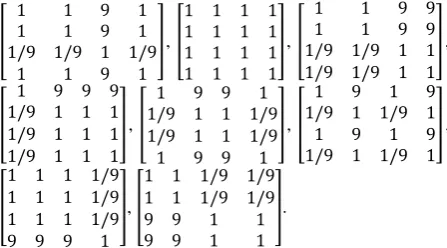
represent the completeness of all alternatives, “1” is used for the present state and “0”is used for absent ones. For the abovementioned eight elements, (1, 1, 0, 1), (1, 1, 1, 1), (1, 1, 0, 0), (1, 0, 0, 0), (1, 0, 0, 1), (1, 0, 1, 0), (0, 0, 0, 1), and (0, 0, 1, 1) are set for alternatives (s1, s2, s3, s4). Following the scale of relative importance proposed by Satty[9, p. 843],
extreme importance in the scale of relative weights is adopted. For each pair of comparison, if the values of completeness are the same in a pair, either 1 vs. 1 or 0 vs. 0, the scale on comparison matrix is 1 (of equal importance).Otherwise, extreme value of 9 (extreme importance) is adopted for 1 vs. 0 and 1/9 for 0 vs. 1. Finally, the comparison matrixes for these eight elements are:
, , , , , , , .
After normalization on columns (all values are divided by the sum of elements in that column), the matrixes become:
, , , , , , .
As a result, the evaluation of alternatives
to these
[image:5.595.316.540.213.337.2]In this case, Evals1 to L1-2, L1-4, 1-1, 1-2, 3-1,
L2-3-2, L2-5-1, and L2-5-2 are 0.3214, 0.25, 0.45, 0.75, 0.45, 0.45, 0.083, and 0.05, respectively. Similarly, Evals2 to these
elements are 0.3214, 0.25, 0.45, 0.083, 0.05, 0.05, 0.083, and 0.05. Evals3 to these elements are 0.0357, 0.25, 0.05, 0.083,
0.05, 0.45, 0.083, and 0.45. Evals4 to these elements are
0.3214, 0.25, 0.05, 0.083, 0.45, 0.05, 0.75, and 0.45.
Finally, the composite relative weights of four alternatives are aggregated via , where GPi is the global
priority of ith element in the lowest level and Evali is the
evaluation of alternative to the ith element.
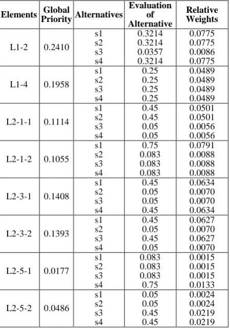
Therefore, the relative weights for s1, s2, s3, and s4 are 0.3856, 0.2032, 0.1650, and 0.2462, respectively. Table 4 shows the computation of relative weights and lists the results in the last column. For example, the relative weight for s1 to L1-2 is the products of global priority to L1-2 and evaluation of alternative s1 to L1-2 is 0.2410×0.3214=0.0775. Finally, the results of relative weights for each alternative from all elements in the lowest level are aggregated as a composite weight. The results are listed in Table 5. For instance, the composite relative weight for s1 is the sum of relative weights of s1 to all elements, listed in the first column: 0.0775+0.0489+0.0501+0.0791+0.0634+0.0627+0.0015+0.00 24=0.3856.
[image:6.595.315.543.349.523.2]Similarly, the composite relative weights for s2, s3, and s4 can be aggregated in the same way. As a result, the composite relative weights for s1, s2, s3, and s4 are 0.3856, 0.2032, 0.1650, and 0.2462, respectively. Based on these weights, the ranking of these four alternatives are s1, s4, s2, and s3, from the top to the bottom.
Table 4. Computation of Relative Weights for Alternatives
Elements Global
Priority Alternatives
Evaluation of Alternative
Relative Weights
L1-2 0.2410 s1 s2 s3 s4
0.3214 0.3214 0.0357 0.3214
0.0775 0.0775 0.0086 0.0775
L1-4 0.1958 s1 s2 s3 s4
0.25 0.25 0.25 0.25
0.0489 0.0489 0.0489 0.0489
L2-1-1 0.1114 s1 s2 s3 s4
0.45 0.45 0.05 0.05
0.0501 0.0501 0.0056 0.0056
L2-1-2 0.1055 s1 s2 s3 s4
0.75 0.083 0.083 0.083
0.0791 0.0088 0.0088 0.0088
L2-3-1 0.1408 s1 s2 s3 s4
0.45 0.05 0.05 0.45
0.0634 0.0070 0.0070 0.0634
L2-3-2 0.1393 s1 s2 s3 s4
0.45 0.05 0.45 0.05
0.0627 0.0070 0.0627 0.0070
L2-5-1 0.0177 s1 s2 s3 s4
0.083 0.083 0.083 0.75
0.0015 0.0015 0.0015 0.0133
L2-5-2 0.0486 s1 s2 s3 s4
0.05 0.05 0.45 0.45
0.0024 0.0024 0.0219 0.0219
Table 5. Composite Relative Weights for Alternatives
Alternatives s1 s2 s3 s4
Composite
Weights 0.3856 0.2032 0.1650 0.2462
Ranking 1 3 4 2
4.4
Validationwith Expert Choice
Finally, the AHP computation of the running example is validated by a popular commercial decision making software packageExpert Choice™(http://www.expertchoice.com/).
When validating the results, distributive mode for aggregating relative weights is set in Expert Choice™. With this mode, the weights are distributed to a group of elements in the same way discussed earlier.The results for the four alternatives are displayed in the upper right window in Expert Choice(see Figure 5).The final composite weights for (s1, s2, s3, s4) are (38.56%, 20.32%, 16.50%, 24.52%).
As a result, external validity of jAHP is accessed by validatingthe same running example using manual approach and Expert Choice.
Fig.5: Results of Incomplete Structure Example in Expert Choice™
Due to the length of this paper, another validation using a running example with complete AHP structure, whose leaf nodes are in the same level, could not be presented. Screenshots of results provided from both jAHP (Fig. A1) and Expert Choice (Fig. A2) are included in Appendix. Same results are obtained through this example as well.
5.
CONCLUSIONS
[image:6.595.56.281.423.747.2]knowledgebase. The knowledgebase would benefit more groups of decision makers with created knowledge and given relative importance of decision-making criteria. As a result, efficient and effective decision-making with a large scale of decision criteria could be reached.
6.
REFERENCES
[1] Aczel, J., and Saaty, T.L. "Procedures for synthesizing ratio judgements," Journal of Mathematical Psychology (27:1) 1983, pp 93-102.
[2] Anane, M., Kallali, H., Jellali, S., and Ouessar, M. "Ranking suitable sites for Soil Aquifer Treatment in Jerba Island (Tunisia) using remote sensing, GIS and AHP-multicriteria decision analysis," International Journal of Water (4:1-2) 2008, pp 121 - 135.
[3] Babic, Z., and Plazibat, N. "Ranking of enterprises based on multicriterial analysis," International Journal of Production Economics (56-57) 1998, pp 29-35.
[4] Hevner, A.R., March, S.T., and Park, J. "Design science in information systems research," MIS Quarterly (28:1) 2004, pp 75-105.
[5] JTree Class, available at:
http://docs.oracle.com/javase/1.5.0/docs/api/javax/swing/ JTree.html
[6] Peffers, K., Tuunanen, T., Rothenberger, M.A., and Chatterjee, S. "A Design Science Research Methodology for Information Systems Research," Journal of Management Information Systems (24:3) 2007, pp 45-77. [7] Ramadhan, R.H., Wahhab, H.I.A.-A., and Duffuaa, S.O. "The use of an analytical hierarchy process in pavement maintenance priority ranking," Journal of Quality in Maintenance Engineering (5:1) 1999, pp 25-39.
[8] Saaty, T.L. The Analytic Hierarchy Process McGraw Hill, NY, 1980.
[9] Saaty, T.L. "Axiomatic foundation of the analytic hierarchy process," Management Science (32:7) 1986, pp 841-855.
[10] Saaty, T.L. "How to make a decision: The analytic hierarchy process," European Journal of Operational Research (48:1) 1990, pp 9-26.
[11] Sinuany-Stern, Z. "Ranking of sports teams via the AHP," Journal of the Operational Research Society (39:7) 1988, pp 661-667.
[12] Vaidyaa, O.S., and Kumar, S. "Analytic hierarchy process: An overview of applications," European Journal of Operational Research (169:1) 2006, pp 1-29.
[13] Zahedi, F.M. "Database management system evaluation and selection decision," Decision Sciences (16:1) 1985, pp 91-116.
[image:7.595.315.542.106.374.2]7.
APPENDIX
Fig. A1: Results of a complete structure example in jAHP.
[image:7.595.316.539.392.570.2]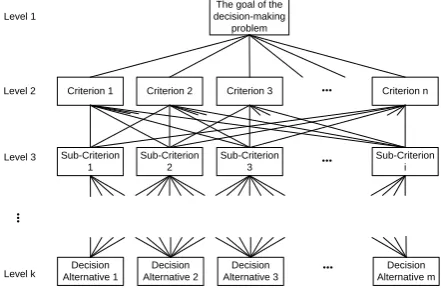
![Table 1. Scale of relative importance [9, p. 843]](https://thumb-us.123doks.com/thumbv2/123dok_us/8091264.784907/2.595.315.544.176.446/table-scale-relative-importance-p.webp)