Forecasting travel time variability

Munich Personal RePEc Archive

Forecasting travel time variability

Eliasson, Jonas

KTH Royal Institute of Technology

2009

FORECASTING TRAVEL TIME VARIABILITY

Jonas Eliasson

Professor Transport Systems Analysis, Director Centre for Transport Studies Affiliation: Centre for Transport Studies, Royal Institute of Technology

Address: Teknikringen 78B, 100 44 Stockholm, Sweden E-mail: jonas.eliasson@infra.kth.se

Presented at the 2009 European Transport Conference

Abstract

In order to incorporate travel time variability in appraisal, methods are needed to predict effects on travel time variability of investments and polity measures. The present study is a first step towards developing such a method. Using data from Stockholm’s automatic camera system for travel time measurements, a relationship is estimated between the standard deviation, the congestion level and various link characteristics. The relationship has been used in a cost-benefit analysis of the planned Stockholm bypass, yielding added benefits of around 15% of the conventional travel time benefits. Moreover, it is shown that that the travel time distribution tends to be less skewed for higher congestion levels, and that the covariance between adjacent links seems to be relatively small. The latter results is important since it makes it possible to approximate route variances as the sum of link variances.

1 INTRODUCTION

As congestion problems are growing more severe in urban regions, the problem of unpredictable travel times is receiving increasing attention. In many cases, this problem is seen as worse than the increased travel time in itself. Infrastructure investments and transport policy measures are often motivated by the need to reduce unexpected delays and unreliable travel times.

Since travel time variability affect people’s utility and their travel behavior, it seems natural to try to include these phenomena in cost-benefit analyses (CBA). In fact, several countries consider doing this or have already. The Netherlands has introduced “reliable travel times” as a goal for transport policy, and is well under way to introduce travel time variability in their CBA methodology (Kouwenhoven, 2005; Hamer et al., 2005). In the UK, there is ongoing work to introduce travel time variability in the CBA part of the appraisal framework (Bates et al., 2004, Department for Transport, 2009).

Travelers’ valuations of travel time variability have been investigated in several studies (see e.g. Hamer et al., 2005, or Eliasson, 2004, for surveys). However, studies that try to provide quantitative methods to forecast travel time variability (or rather, effects on variability of investments or policy measures) are still rather scarce. The present study is an attempt to develop such a method. The task at hand is analogous to developing volume-delay functions: just as volume-delay functions describe the relationship between the traffic volume, capacity and travel time on a link, the intention is to try to develop a function that describes the relationship between travel time, free-flow travel time and the standard deviation of travel time.

2 ABOUT TRAVEL TIME VARIABILITY

Travel time variability is the random, day-to-day variation of the travel time that arises in congested situations even if no special events (such as accidents) occur. If congestion is severe, this variation may be significant. The variability means that many travelers must use safety margins in order not to be late. In some cases, the margin will turn out to be insufficient, and the traveler will be late nevertheless. In the former case, an additional disutility (beyond that measured by pure mean travel time) arises since effective travel time can be said to be greater than actual mean travel time. In the latter case, the lateness will cause some sort of additional disutility. The social loss caused by the travel time variability is the sum of those two disutilities.

2.1 Valuing travel time variability

Many valuation studies assume a (reduced-form) utility function on the form

u = t + c + 

There are also studies that estimate schedule delay costs directly, i.e. the additional costs travelers encounter when they start earlier to reduce the risk of being late and the occasional “lateness penalty” when the travel time turned our to be longer than expected. Such studies usually use (variants of) the framework proposed by Vickrey (1969), Small (1982) and Noland and Small (1995). Fosgerau and Karlström (2009), extending results by Noland and Small (1995) and Bates et al. (2001), show that if the lateness penalty (arrival after the preferred arrival time) is linear, the departure time can be chosen freely and the travel time distribution is independent of departure time (although they show that this condition is of less practical importance), the indirect utility function will be on the form above. An important caveat, though, is that the relative weight of the standard deviation () will depend on the standardized travel time distribution. Standard deviation valuations that have been obtained in one context can thus not be directly transferred to another context with a different standardized travel time distribution.

The question of proper valuation of travel time variability is not the main focus of the current paper. The main motivation for it, however, is that it currently seems that the most tractable way of introducing travel time variability in cost-benefit analyses is using the mean-variance approach (or a variant thereof) – and hence, a way to forecast travel time variability is needed.

2.2 Measures of travel time variability

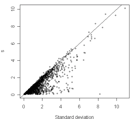
There are several ways to quantify travel time variability. We will use two similar measures: the standard deviation of travel time (denoted ) and the difference between the 90- and 10-percentile, scaled by the factor 2.56 (denoted s). The factor 2.56 is chosen so that if the travel time is normally distributed, the measures will coincide. If the travel time is symmetrically distributed, s and  will only differ by a scale factor. (As will be shown later, the distribution of the travel time will tend to be relatively symmetric for high congestion levels.) The main advantage with using s during estimation is that the estimated relationship between congestion and travel time variability will be more precisely estimated, since s, unlike , is not sensitive to occasional, “rare” incidents, beyond the 90th _{percentile. Obviously, an estimated}

Figure 1. Standard deviation compared to s.

The figure above shows that s and  lie close in the majority of cases, especially for higher standard deviations. As expected, when the two measures differ, it is the standard deviation that is higher: this depends on “rare” events causing high travel times, increasing the tail beyond the 90th

percentile and hence increasing  but not s.

As it turns out, estimations work better (in terms of R2 _{and parameter}

significance) when using s as a dependent variable than when using the standard deviation . This seems to depend on the fact that  is sensitive to outliers in the far right tail of the distribution – which may be due to rare, occasional incidents, or due to measurement errors; it is virtually impossible to tell. Since s and  “should” coincide for high congestion and variability (and mostly do), it is an attractive option to use s as a measure of the variability rather than the standard deviation. s can also be viewed as a “proxy” for the standard deviation, that is less sensitive to measurement errors and “irrelevant” incidents (road work, say). Estimation results are presented both for s and .

3 DATA

The data used comes from the automatic travel time measurement system in Stockholm. Travel times are measured continuously through a camera system, where pictures of number plates are taken when vehicles enter and leave each link. The number plates are then matched together, and the travel time for each vehicle is calculated. Each period of 15 minutes, the median travel time on the link is calculated (after a filtering process to weed out various sorts of errors). The median is used rather than the average in order not to let vehicles stopping along the link (buses, shoppers) affect travel time measurements.

Travel times are measured on 92 streets and roads in and around central Stockholm. During the period we studied, measurements worked properly on 41 of these links. All the links can be characterized as “urban” roads, i.e. they are neither highways nor small, “local” streets. Typically, they have two lanes in each direction (sometimes only one) – remember that Stockholm is a European city, and, compared to e.g. typical US conditions, even fairly large urban roads are narrow and seldom have more than two lanes. Around two thirds of the links have a speed limit of 50 km/h, and the rest have 70 km/h. Traffic volumes vary between 15 000 and 50 000 vehicles per day (summing both directions). Lengths vary from 300 meters to 5 km, so most links also contain a few intersections, mostly signaled.

We used data from Monday-Thursday1 _{during three time periods: the spring of}

2005 (week 15-20), the fall of 2005 (September 1 – November 29) and the spring of 2006 (week 14, 16-202_{). For each link and time period, we calculated}

average travel time and the standard deviation of the travel time for each 15 minutes period between 6.30 and 18.30 – hence, each link produced 3*48 “observations” of mean travel time and standard deviation (there are 48 quarters between 6.30 and 18.30). Calculating the standard deviation across each time period means implicitly assuming that each of three time periods is “homogeneous” in the sense that variability during that time period is random from the traveler’s point of view – in particular, that there are no foreseeable season effects during the course of the time period. This assumption is verified by checking that there are no discernible trends in traffic volumes or travel times during the time periods (as opposed to if we had, for example, extended the spring time period into the summer, when traffic first increases and then drops sharply after Midsummer). In the estimations, we will present both estimations on the three time periods separately and on the whole pooled data set.

That we split the day into 15-minute periods is an implicit assumption that this is the relevant “time resolution” that travelers base their decisions on. In general, the more coarse this “time resolution” is chosen, the larger will the calculated variability be (and vice versa), since the variability of travel times across the day will affect the standard deviation. Our choice is essentially only motivated by intuition: it seems reasonable that most travelers will “know” the

variations in (expected) travel conditions on a 15-minutes basis. Investigating this further would certainly be worthwhile.

4 INVESTIGATING TRAVEL TIME VARIABILITY

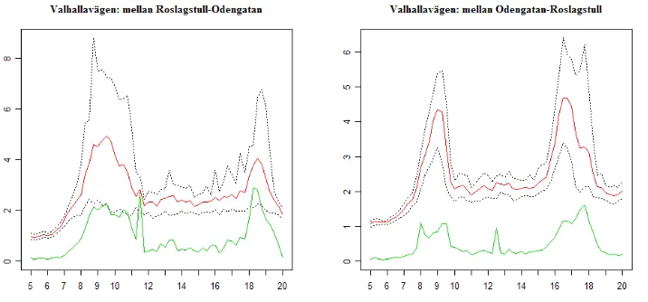
Before we present estimation results, it is useful to get some qualitative feel for the standard deviation. The diagrams below show mean travel time (red) and 10- and 90-percentiles for a few links. A striking feature is the large variation of travel time – during the 10% “best” days, travel times are close to free flow even during rush hours, while the 10% “worst” days, travel times may be twice as long than average travel times (or more), and at least four times as long as the 10% “best” days.

Figure 2. An example of travel times: Valhallavägen (two directions). Red is average travel time, black dotted lines are 10- and 90-percentiles of the travel time. Green is the standard deviation ().

Figure 3. Another example of travel times: the Central bridge (two directions). Red is average travel time, black dotted lines are 10- and 90-percentiles of the travel time. The green, jagged line is the standard deviation () and the blue, less jagged line is s, the (scaled) distance between the 90- and 10-percentile (see text).

This particular link was also chosen to show the difference between  and s. In particular on the left pane,  is apparently disturbed by various large outliers – due to e.g. measurement errors or incidents. Although the data has been checked as far as possible to correct it, it is hard to weed out all outliers – especially in a study of this type, where it is the variation itself that we want to study. But from the figure, it is apparent that s is more “stable” than , and it should come as no surprise that the estimated relationships for s show higher significance than those for .

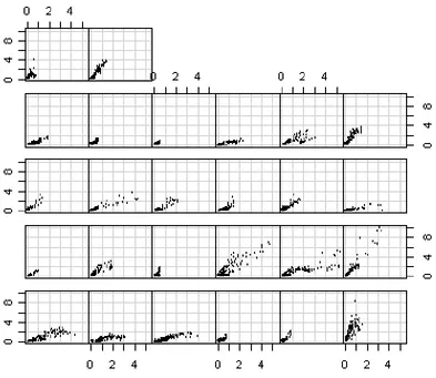
From the figures above, it seems apparent that there is a relationship between congestion (i.e., travel time longer than the free-flow travel time) and travel time variability. The diagrams below show relative standard deviation ( divided by free-flow travel time) on the y-axis vs. relative increase in travel time (actual travel time divided by free-flow travel time) for 26 links. Each “dot” is one 15-minute period between 6.30 and 18.30.

Figure 4. Relative standard deviation vs. relative increase in travel time for 26 links.

slope and trying to explain why it differs is one of the main tasks of this study, but before we show estimation results, we need to digress a little and investigate the distribution of travel times, and how variability is affected by queue build-up and dissipation.

5 THE DISTRIBUTION OF TRAVEL TIMES

An interesting question is how travel times are distributed over multiple days. That is, if you measure the travel time on a certain link at a certain time of day several days3 _{- what will the distribution of these measurements look like? In}

particular: is it skewed or symmetric? The answer to this has implications for how stated choice experiments are formulated, and as noted in the introduction, the shape of the travel time distribution will affect the valuation of the standard deviation ( in the introduction).

An initial guess might be that the distribution of travel times might be “skewed to the right”, i.e. deviations “upwards” – longer travel times than the median – is larger than deviations “downwards”. It turns out that this is only partially correct. First, there is a large variation in terms of skewness, especially for low congestion levels. For higher congestion levels, skewness decreases to the point where the travel time is distribution is almost symmetric. The rest of this section is devoted to show this.

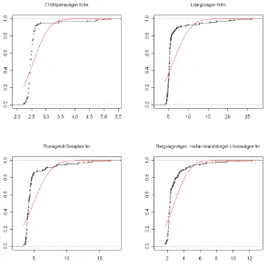
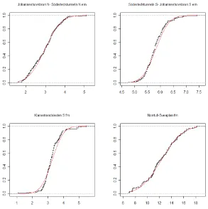
The pictures below show a few examples of cumulative distributions of travel times. Every “dot” shows a certain 15-minute period a certain day. The red line shows a cumulative normal distribution with the same mean and standard deviation. “fm” means AM peak (8.00-9.00 AM) and “em” means PM peak (5.00-6.00 PM).

Figure 5. Examples of skewed travel time distributions (travel time in minutes on the x-axis, cumulative frequency during 1 rush hour on the y-axis).

These links are typical examples of links with low congestion. Most days, travel times are just a little above free-flow travel time, only getting longer in a few cases. Then, on the other hand, the travel time may be considerably longer – in some cases three or five times as long as the free-flow travel time. One may hypothesize that these cases are due to accidents, road work or bad weather (snow, heavy rain etc.). From the travelers’ viewpoint, travel time is “almost deterministic” – the travel time will be the same 90-95% of the trips. Only for the remaining 5-10%, the travel time will be longer.

Figure 6. Examples of normally distributed travel times.

These travel time distributions are clearly almost exactly normally distributed. From a travelers’ viewpoint, the main difference is that travel times are clearly random – very different from day to day. (Interestingly, traffic volumes do not vary much – typically a few percent from day to day.)

Figure 7. Cumulative travel time distributions, spring 2005 and spring 2006.

The figures above give anecdotic support for the statement that travel time distributions are skewed for moderate levels of congestion (and variability), while it tends to be symmetrically distributed (normally, to be precise) for high levels of congestion (and variability).

To show this more formally, we use the standard definition of skewness: S = E([X-m]3_)/3 _{(m is the mean and}  _{the standard deviation). If S is 0, then}

the distribution is symmetric. If S is negative, it is skewed to the left, and vice versa for positive S.

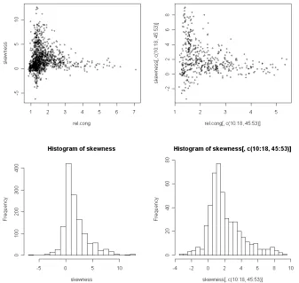
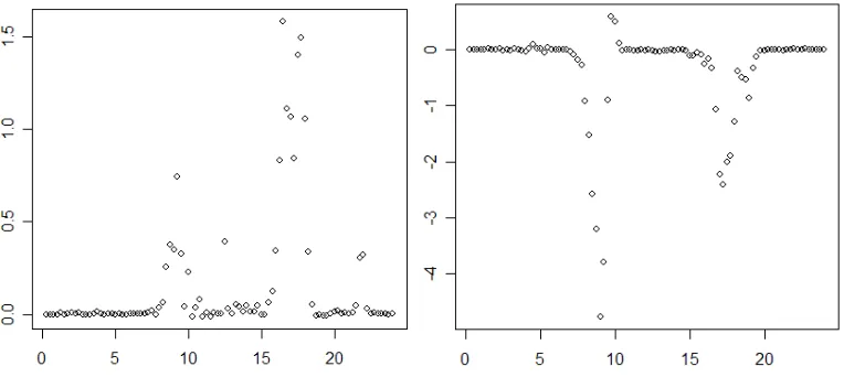
The diagram below to the right shows (on the y-axis) the skewness for the travel times during 1 hour periods between 5 AM and 9 PM for 41 links. The skewnesses are plotted against the relative increase in travel time (actual travel time divided by free-flow travel time) – a measure of congestion. To the left, skewness for 15-min distributions during rush hours are shown.

Figure 8. Skewness of travel time distribution (y-axis) vs. relative increase in travel time (x-axis). Left: one-hour distributions 5:00-21:30, different for the three measuring periods (spring 05, fall 05, spring 06). Right: 15-min distributions during rush hours (7-9, 16-18), aggregated over measuring periods. Below: corresponding histograms.

Since we are primarily interested in congested conditions, this is a convenient result in stated choice contexts: it is much harder to present highly skewed travel time distributions to travelers in a comprehensible way than it is to present symmetric distributions with moderately long tails.

6

VARIABILITY DURING QUEUE BUILD-UP AND

DISSIPATION

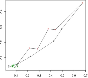
Bates et al. (2002) studied how the variability on highways changed during the day. From a simple random-capacity bottleneck model, they show that the variability can be expected to be higher during queue build-up than during queue dissipation. They also report that this phenomenon can be found in measurement data. The same result is reported, and a general proof is provided, in Fosgerau (2008). This phenomenon is often visible in our material as well – though not always. In the diagram below, relative increase in travel time is plotted (x-axis) versus relative s (s divided by free-flow travel time) (y-axis). Colors show time of day: black circles are observations through 8.45, red circles through 9.45, and then green circles.

0.1 0.2 0.3 0.4 0.5 0.6 0.7

0

.1

0

.2

0

.3

0

.4

Figure 9. Relative travel time variability (y-axis) vs. relative increase in travel time (x-axis) for different 15-minute timer periods.

Relative variability is roughly proportional to relative increase in travel time (which can be interpreted as “congestion”). But during queue dissipation – from 9.00, when the red circles start – the variability is higher than during queue build-up, although the congestion is the same. During mid-day (from 10.00 onwards), both congestion and variability are negligible.

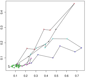
increasing congestion, and then decreases again with decreasing congestion, but at a higher level. Mid-day (green) and evenings (purple) , both congestion and variability are negligible.

0.1 0.2 0.3 0.4 0.5 0.6 0.7

0

.1

0

.2

0

.3

0

.4

Figure 10. Relative travel time variability (y-axis) vs. relative increase in travel time (x-axis) for successive 15-minute time periods.

The diagrams below show more examples (all from the morning peak). The phenomenon is not always as apparent, but enough important to be accounted for during estimation.

0.00 0.05 0.10 0.15 0.20 0.25 0.30

0.

05

0.

10

0.

15

0.0 0.2 0.4 0.6 0.8 1.0 1.2

0

.10

.20

.30

.40

.50

.60

Figure 11. Relative travel time variability (y-axis) vs. relative increase in travel time (x-axis) for successive 15-minute time periods.

7 ESTIMATION

RESULTS

As was illustrated above, there is a positive correspondence between variability and “congestion” (measured as relative increase in travel time throughout). It turns out that modeling this correspondence with a log-log function works best (in terms of R2_{) – we also tried linear and log-linear}

functions. A log-log function also has the desirable property that the standard deviation is guaranteed to be positive when we use the estimated relationship for forecasting.

Two types of models are presented: one with the standard deviation  as the dependent variable, and one with s (the difference between the 90th _percentile

and the 10th _{percentile, scaled to coincide with the standard deviation if the}

distribution is normal) as the dependent variable. As noted above,  is more sensitive to outliers (rare incidents or possibly measurement errors), so the  models have somewhat less explanatory power (in terms of R2 _{and parameter}

significance). Obviously, “rare” incidents are still relevant for the travel time distribution we are studying – but there is little hope that we will be able to model the frequency and impact of such random incidents in the type of model and data at hand here. The parameters of the model types are remarkably similar, however.

The variables included in the model are

- mean travel time (t)

- relative increase in travel time over free-flow travel time t0 (t/t0-1)

- length of the link in kilometers (L)

- dummy variable for “time of day” (ToD). The parameter for mid-day is

- dummy variable for the speed limit (speed). The parameter for speed limit 50 km/h is normalized to zero.

The estimated formula is:

       _      

 * * * * 1

0 t t t L speed ToD

where  is a constant. Further, a set of models where  was replaced with s (the 90-10-percentile distance) was estimated. Separate models were estimated for the three time periods – spring 2005, fall 2005, spring 2006 – and then one model for the pooled data. The results are shown in the table below. all years std. error t-stat. spring 2005 std. error t-stat. fall 2005 std. error t-stat. spring 2006 std error t-stat.

(Intercept)  -1.50 0.03

-57.8 -1.27 0.05

-26.7 -1.69 0.04

-44.4 -1.46 0.05 -30.0 log(travel

time)  1.09 0.02 48.3 1.04 0.04 26.5 1.09 0.03 31.8 1.02 0.04 23.6 log(congestion

index)  0.52 0.01 48.8 0.56 0.02 27.6 0.52 0.02 32.1 0.48 0.02 26.0

log(length)  -0.28 0.02

-14.4 -0.23 0.03 -6.7 -0.29 0.03

-10.2 -0.26 0.04 -6.7 after PM peak

ToD 0.14 0.02 5.5 0.02 0.04 0.5 0.23 0.04 5.8 0.17 0.05 3.7 after AM peak 0.18 0.03 7.0 0.02 0.04 0.5 0.31 0.04 7.5 0.22 0.05 4.7 before PM

peak ToD 0.00 0.02 0.1 -0.13 0.04 -3.2 0.06 0.04 1.5 0.10 0.05 2.2 before AM

peak ToD 0.02 0.02 0.8 -0.05 0.04 -1.4 0.06 0.03 1.9 0.04 0.04 1.1 speed limit 70

km/h speed 0.27 0.02 13.3 0.27 0.03 7.9 0.34 0.03 10.3 0.21 0.04 5.6

Multiple

R-Squared 0.61 0.68 0.73 0.61

all years std. error t-stat. spring 2005 std. error t-stat. fall 2005 std. error t-stat. spring 2006 std error t-stat.

(Intercept)  -1.97 0.02

-92.3 -1.60 0.04

-41.5 -2.10 0.03

-65.8 -2.15 0.04 -55.1 log(travel

time)  1.23 0.02 66.5 1.04 0.03 32.7 1.20 0.03 41.9 1.37 0.03 39.1 log(congestion

index)  0.46 0.01 53.4 0.58 0.02 34.7 0.51 0.01 37.2 0.35 0.01 23.4

log(length)  -0.32 0.02

-20.1 -0.15 0.03 -5.3 -0.31 0.02

-13.1 -0.47 0.03 -15.2 after PM peak

ToD 0.18 0.02 8.7 0.03 0.03 0.9 0.24 0.03 7.3 0.26 0.04 7.1 after AM peak 0.18 0.02 8.4 0.09 0.04 2.6 0.26 0.03 7.6 0.18 0.04 4.6 before PM

peak ToD 0.06 0.02 3.1 -0.07 0.03 -2.1 0.11 0.03 3.4 0.16 0.04 4.4 before AM

peak ToD 0.10 0.02 5.8 0.05 0.03 1.7 0.18 0.03 6.2 0.09 0.03 2.8 speed limit 70

km/h speed 0.12 0.02 7.4 0.08 0.03 2.9 0.24 0.03 8.9 0.09 0.03 2.9

Multiple

R-Squared 0.76 0.77 0.81 0.72

- The parameters do not change much across time periods, despite very different traffic conditions in terms of traffic and congestion levels due to seasonal variations and, above all, the congestion charges in the spring of 2006. Although a formal test rejects the hypothesis that the data can be combined into a pooled model, that finding should be interpreted with caution, since the data sets are so large. In particular, the parameters for the  models seem very stable. The parameters for the  models seem to be somewhat more stable than those for the s models, despite the fact that the latter models have better explanatory power in terms of R2_.

- The standard deviation is almost proportional to the mean travel time (the exponent is just above 1), proportional to the square root of the congestion index and proportional to the length raised to the power of -0.3. These results seem to be stable across time periods.

- The s model parameters are a little less stable across time periods. A recurrent finding is that all models have + = 1.7, i.e. for high congestion levels (t>>t0), s increases as (travel time)1.7 in all s models.

- The time-of-day parameters for “after AM peak” and “after PM peak” pick up the “looping” behavior that causes the standard deviation to be higher during the queue dissipation phase.

- A higher speed limit increases the standard deviation. It is unclear whether this is because of the speed limit itself or whether this is a proxy for various other characteristics of the road. Considering the fact that no other road characteristics were significant (see the list below), it seems likely that it is in fact the speed limit in itself that causes the increase in standard deviation.

Variables that were tried in the estimation but eventually were excluded because they were insignificant were.

- number of intersections on the link

- free-flow travel time (although it is included in the “congestion measure”)

- number of lanes

- “Emme/2-classification” – a classification of all links describing its size and function

- the “degree of distortion” of the link, as coded in the emme/2. This is used in the volume/delay functions, and describes factors as curvature, parked cars, intersection types etc.

8 ARE TRAVEL TIMES ON ADJACENT LINKS CORRELATED?

An interesting question is whether the travel times on adjacent links are correlated. More precisely: if the travel time on a certain link at a certain time of day is higher than usual – will the travel time on another, adjacent link tend to be higher or lower than usual, or is it unaffected?

deviations be ij and jk. The standard deviation for the whole (two-link) route (i,k) is





jk ij

ik 2Covt ,t

2

2  

   

Hence, if travel times are uncorrelated, then – and only then – we can just add the variances to get the variance for the whole route.

There are several arguments that suggest that travel times on adjacent links should be positively correlated. If the variability of the travel times stems from variations in the traffic volume, then the same underlying variability source will affect both links similarly. The same is true for incident-related variability. A third reason is that a queue that builds up on one link will tend to “spill over” onto previous links.

But there are also arguments that suggest that travel times on adjacent links might be negatively correlated. A link that lies “downstream” from a bottleneck (an overloaded intersection, typically) will get lower traffic flow those days when the bottleneck is more than usually overloaded. This will lead to higher travel times upstream from the bottleneck but lower travel times downstream from the bottleneck – and hence, negatively correlated travel times.

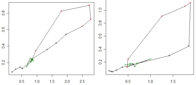
In our material, there are five pairs of adjacent links. The diagrams below show two examples of how the covariance of two of the five pairs varies across the day. As it turns out, three of the five pairs have positively correlated travel times (one of which is shown to the left), one pair has negatively correlated travel times (shown to the right), and one pair has positively correlated travel times during the morning peak, but negatively correlated travel times during the afternoon peak.

Figure 12. Relative covariance (y-axis) across the day (hours are shown on x-axis).

The pair with negatively correlated travel times fits the hypothesis above: the second link in the pair lies downstream from a bottleneck where several highly congested links meet in a roundabout.

would be virtually intractable to compute covariances for each pair of links in the whole network, especially since data is limited.

The diagrams below show the correct standard deviation for a pair of adjacent links on the x-axis, and the square root of the summed link variances on the y-axis – that is, what we get if we assume uncorrelated link travel times, and omit the covariance term from the formula above. Dots on the straight line are a perfect fit; dots below the line mean that the total standard deviation for the link pair is underestimated if the covariance term is omitted.

Figure 13. True standard deviations for link pairs (x-axis) vs. the approximated standard deviation when covariance is ignored (y-axis).

In most cases, the standard deviation is moderately underestimated when the covariance term is omitted. The table below show the percentage error during morning and afternoon peak hours for the five link pairs.

Link pair Time period Mean error

Mean absolute error Roslagstull-Odengatan and

Odengatan-Lidingövägen

7:00-9:30 -5% 6%

16:00-18:30 7% 8%

Same, other direction

7:00-9:30 -6% 8%

16:00-18:30 -19% 20%

Islandstorget-Brommaplan and Brommaplan-Stora Mossen

7:00-9:30 8% 8%

16:00-18:30 8% 9%

Same, other direction

7:00-9:30 -12% 12%

16:00-18:30 0% 4%

Sveaplan-Odengatan and Odengatan-Sergels torg

7:00-9:30 0% 7%

16:00-18:30 -13% 13%

occurs when link variances are summed without the covariance term should be tolerable.

9 CASE STUDY: THE VALUE OF VARIABILITY REDUCTION

The western bypass is a planned major road investment in Stockholm. During the spring of 2006, we conducted the cost-benefit analysis of the bypass. It was decided by the National Road Administration that travel time variability should be included into the CBA, as a test before a decision to include it in standard CBA.

The formula above was implemented as an Emme/2 macro, using travel times and free-flow travel times from the Emme/2 network as input.

Since this was only a test, and there was a pressing time limit, a few simplifications were made. First, all vehicles were assumed to have the same value of time. Second, only conditions during morning peak were considered, and this was then scaled to a value for the entire day. This consumer surplus of reduced variability W was then calculated using rule-of-a-half:







 ij

ij ij ij

ij T

T

W 1 0

1 0

2  



where Tij is flow between the OD pair (i,j), 0 and 1 refer to the situations with/without the investment,  is the value of time and  is the scale factor from morning peak hour to the entire day. Calculating ij for OD pair (i,j), we

assumed that standard deviations were independent across links.

Net present values Alt. 1 (west)

Alt. 2 (east)

Producer surplus 333 243

Budget effects 1764 1773

Travel time 20 973 21 677

Travel cost 1971 2480

Freight costs 1148 1257

Emissions 643 1612

Traffic safety 1018 1561

Investment costs (incl. marg. cost of public funds etc.) -19570 -19570

Maintenance -3232 -3031

Reduced travel time variability 2912 3420

Total benefits excl. reduced variability 24 632 27 583 Total benefits incl. reduced variability 27 544 30 177 Net present value ratio incl. reduced variability 0,26 0,41 Net present value ratio incl. reduced variability 0,41 0,54

Table 1. Costs and benefits of a western bypass, net present values.

What is interesting about this table in the present context is that the value of reduced travel time variability is quite significant – about 15% of the total value of travel time savings. Thus, it seems that it would be worthwhile to continue the work of including travel time variability into CBAs, at least in urban contexts.

This figure can be compared with a rough rule-of-thumb: The average ratio between standard deviation and mean travel time for the links in our data set is approximately 0.2. With a valuation of standard deviation of 0.9*(value of time), this would mean that adding reliability benefits would mean an increase of time benefits of 18%. However, this does not take into account that more of the traffic occurs during the most congested hours. On the other hand, the links in the data set is more congested than the average link in Stockholm. Correcting for the former approximation would increase the rough of-thumb, while taking the second fact onto account would decrease it. As a rule-of-thumb, it is obviously far too simplified; but as a check of the magnitude, it has some value.

10 CONCLUSIONS

the effects on variability of investments or policy measures. The work presented here is meant to be a step towards filling that gap.

The central contribution of the paper is the estimation of a relatively stable relationship between the travel time variability on a link, its travel time, its congestion index and a number of other parameters. The estimated relationship gains more credibility from the fact that the parameters appear stable when compared across three distinct time periods with different traffic and congestion conditions.

Other findings from the data analyzed in the paper are

- The travel time variability does not only depend on the congestion level, but also on whether the queue is in its build-up or dissipation phase. For a given congestion level (in terms of increased travel time),variability will be higher.

- The skewness of the travel time distribution appears to decrease when congestion increases. For high congestion levels, skewness appears to be almost negligible.

- In order to calculate the standard deviation of the origin-destination travel times, it is for practical reasons virtually necessary to assume link travel times are independent. Based on a limited number of adjacent link pairs, it seems as though this simplification does not introduce a serious error in the calculation.

- Travel time variability benefits may be substantial. In a case study of a bypass around Stockholm, travel time variability benefits amounted to around 15% of conventional travel time benefits.

From a policy point of view, a seemingly trivial conclusion is that attacking congestion is more important than is apparent from just the increase on average travel times caused by the congestion. In other words, investments and policy measures that decrease congestion levels are worth more than the face value of travel time savings valued in the conventional way. Even if the CBA methodology may yet not be developed to the point where travel time variability benefits can safely be included in a routine manner, the message to policy makers is clear: that congestion creates costs for the society well above the mere time losses it creates, if that time loss is valued in the conventional way.

11 ACKNOWLEDGMENTS

Financial support from VINNOVA (The Swedish Governmental Agency for Innovation Systems) and the National Road Administration is gratefully acknowledged.

Bates, J., Black, I., Fearon, J., Gilliam, C., and Porter, S. (2002) Supply models for use in modeling the variability of journey times on the highway network. Presented at the European Transport Conference, 2003.

Bates, J., Fearon, J. and Black, I. (2004) Frameworks for Modeling the Variability of

Journey Times on the Highway Network. Department of Transport, UK.

Bates, J., J. Polak, P. Jones, A. Cook (2001) The valuation of reliability for personal travel. Transportation Research E37, 191-229.

Börjesson, M. (2006) Departure time modeling: applicability and travel time uncertainty. PhD Thesis, KTH, Stockholm.

Department for Transport (2009) The Reliability Sub-Objective: TAG Unit 3.5.7. Available at http://www.dft.gov.uk/webtag/docs/expert/economy-objective/3.5.7.pdf.

Eliasson, J. (2004) Car drivers’ valuations of travel time variability, unexpected delays and queue driving. Presented at the European Transport Conference, 2004.

Fosgerau, M. (2008) On the relation between the mean and variance of delay in dynamic queues with random capacity and demand. Working paper, available at http://mpra.ub.uni-muenchen.de/11994/.

Fosgerau and Karlström (2009) The value of reliability. Transportation Research B, in press. doi:10.1016/j.trb.2009.05.002.

Hamer, R., de Jong, G., Kroes, E. and Warffemius, P. (2005) The value of reliability

in transport. Provisional values for the Netherlands based on experts’ opinion.

RAND Europe.

Hollander, Y. (2005) The attitudes of bus users to travel time variability. Presented at the European Transport Conference, 2005.

Kouwenhoven, M., Schoemakers, A., van Grol, R., and Kroes, E. (2005)

Development of a tool to assess the reliability of Dutch road networks. Presented

at the European Transport Conference, 2005.

Noland, R.B., Small, K. (1995) Travel time uncertainty, departure time and the cost of the morning commute. 74th _{meeting of the TRB.}

Small, K. (1982) The scheduling of consumer activities: work trips. American

Economic Review72, 172-181.

van Amelsfort, D.H. (2005) Valuation of uncertainty in travel time and arrival time: some findings from a choice experiment. Presented at the European Transport Conference, 2005.

Vickrey, W.S., (1969) Congestion theory and transport investment. American