Identifying common dynamic features in stock returns

Munich Personal RePEc Archive

Identifying common dynamic features in

stock returns

Caiado, Jorge and Crato, Nuno

April 2009

Identifying common dynamic

features in stock returns

Jorge Caiado and Nuno Crato

CEMAPRE, Instituto Superior de Economia e Gestão,

Technical University of Lisbon,

Rua do Quelhas 6, 1200-781 Lisboa, Portugal.

Tel. +351 213 922715 Fax +351 213 925846 Email (corresponding author): [email protected]

Abstract

This paper proposes volatility and spectral based methods for cluster analysis of stock returns. Using the information about both the estimated parameters in the threshold GARCH (or TGARCH) equation and the periodogram of the squared returns, we compute a distance matrix for the stock returns. Clusters are formed by looking to the hierarchical structure tree (or dendrogram) and the computed principal coordinates. We employ these techniques to investigate the similarities and dissimilarities between the "blue-chip" stocks used to compute the Dow Jones Industrial Average (DJIA) index.

Keywords: Asymmetric e¤ects; Cluster analysis; DJIA stock

returns; Periodogram; Threshold GARCH model; Volatility.

1

Introduction

Cluster analysis of …nancial time series plays an important role in several areas of application. In stock markets, the examination of mean and variance correlations between asset returns can be useful for portfolio diversi…cation and risk management purposes. In international equity market analysis, the identi…cation of similarities in index returns and volatilities can be useful for grouping countries. Finally, the existence of asymmetric cross-correlations and dependences in asset returns can be of interest for …nancial research.

used for analyzing the structure of the asset returns. A …rst technique is the principal component analysis (PCA), which is concerned with the covariance structure of asset returns and can be used in dimension re-duction (Tsay, 2005). A second technique is the factor model for asset returns that uses multiple time series to describe the common factors of returns (see, e.g., Zivot and Wang, 2003, for further discussion). A third technique is the identi…cation of similarities in asset return volatil-ities using cluster analysis (see, for instance, Bonanno, Caldarelli, Lillo, Miccieché, Vandewalle and Mantegna, 2004).

A fundamental problem in clustering economic and …nancial time se-ries is the choice of a relevant metric. Mantegna (1999), Bonanno, Lillo and Mantegna (2001), among others, used the Pearson correlation coe¢-cient as similarity measure of a pair of stock returns. Although this met-ric can be useful to ascertain the structure of stock returns movements, it has two problems. Firstly, it does not take into account the stochastic volatility dependence of the processes – in fact, two processes may be highly correlated and have very di¤erent internal stochastic dynamics. Secondly, it cannot be used directly for comparison and grouping stocks with unequal sample sizes – this is a common problem of most exist-ing nonparametric-based methods, as discussed, for instance, in Caiado, Crato and Peña (2009).

In this paper, we introduce a distance measure between the threshold GARCH model parameters of the return series. In order to also capture the spectral behavior of the time series, we suggest combining the pro-posed statistic with a periodogram distance measure for the squared returns. Finally, we suggest using a hierarchical clustering tree and a multidimensional scaling map to explore the existence of clusters. We apply these steps to investigate the similarities and dissimilarities among the “blue-chip” stocks of the Dow Jones Industrial Average (DJIA) in-dex.

The remaining sections are organized as follows. Section 2 provides volatility and spectral based distances for clustering asset returns. Sec-tion 3 describes the data and explores the univariate statistics. SecSec-tion 4 presents the empirical …ndings on the cluster analysis. Section 5 covers the multidimensional scaling results. Section 6 summarizes and con-cludes.

2

Volatility and spectral based distances

shock than a positive shock of the same magnitude.

A univariate volatility model commonly used to allow for asymmetric shocks to volatility is the threshold GARCH (or TGARCH) model (see Glosten, Jagannathan and Runkle, 1993 and Zakoian, 1994). The simple TGARCH(1,1) model assumes the form

"t=zt t, (1)

2

t =!+ 2t 1+ "t2 1+ "2t 1dt 1, (2) where fztgis a sequence of independent and identically distributed ran-dom variables with zero mean and unit variance; dt= 1 if "tis negative, and dt = 0 otherwise. The volatility may either diminish ( < 0), rise

( > 0), or not be a¤ected ( 6= 0) by negative shocks or "bad news" ("t 1 < 0 ). Good news have an impact of while bad news have an impact of + . The persistence of shocks to volatility can be given by

+ + =2.

Nelson (1991) also proposed an heteroskedasticity model to incorpo-rate the asymmetric e¤ects between positive and negative stock returns, called the exponential GARCH (or EGARCH) model, in which the lever-age e¤ect is exponential rather than quadratic.

In real applications,ztis often assumed to follow a "fat-tailed"

distri-bution, as it can be given by the Generalized Error Distribution (GED). The GED has probability density function

f(z) = vexp [ 0:5jz= j

v

]

2(1+1=v) _(1=v) ;0< v 1; 1< z <+1; (3) wherev is the tail-thickness parameter, ( )is the gamma function, and

= 2

( 2=v) _(1=v)

(3=v)

0:5

. (4)

When v < 2, fztg is fat-tailed distributed. When v = 2, fztg is

normally distributed. When v > 2, fztg is thin-tailed distributed. For details, see, e.g., Tsay 2005, p. 108.

We now introduce a distance measure for clustering time series with similar volatility dynamics e¤ects. Let rx;t = logPx;t logPx;t 1 de-note the continuously compounded return of an asset x from timet 1

to t (ry;t is similarly de…ned for asset y). Suppose we …t a common

TGARCH(1,1) model to both time series by the method of maximum likelihood assuming GED innovations. Let Tx = (_bx;bx;bx;bvx)0 and Ty = (by;by;by;bvy)0 be the vectors of the estimated ARCH, GARCH,

A Mahalanobis-like distance between the dynamic features of the return series rx;t and ry;t, called the TGARCH-based distance, can be de…ned by

dT GARCH(x; y) = q(Tx Ty)0 1_{(Tx Ty), (5)}

where =Vx+Vy is a weighting matrix. This way, the matrix weights the parameters taking into account the uncertainty in their estimation. The distance (5) takes into account the information about the stochastic dynamic structure of the time series volatilities and allows for unequal length time series.

We can also use methods based on the periodogram ordinates or the autocorrelations lags of the squared returns. The spectrum of the squared return series provides useful information about the time series behavior in terms of the ARCH e¤ects.

LetPx(!j) = n 1_jPn

t=1rt;xe it!jj2be the periodogram of the squared return series,r2

x;t, at frequencies !j = 2 j=n, j = 1; :::;[n=2](with [n=2]

the largest integer less or equal to n=2). Let s2

x be the sample variance

of rx;t (similar expression applies to asset y)

The Euclidean distance between the log normalized periodograms (Caiado, Crato and Peña, 2006) of the squared returns of x and y is given by

dLN P(x; y) =

v u u t

[_Xn=2]

j=1

log Px(!j)

s2

x

log Py(!j)

s2

y

2

, (6)

or, using matrix notation,

dLN P(x; y) =

q

(Lx Ly)0(Lx Ly). (7)

where Lx and Ly are the vectors of the log normalized periodogram

ordinates of r2

x;t and ry;t2 , respectively.

Since the parametric features of the TGARCH model are not neces-sarily associated with all the periodogram ordinates, the parametric and nonparametric approaches can be combined to take into account both the volatility dynamics and the cyclical behavior of the return series, that is

dT GARCH LN P(x; y) = 1

q

(Tx Ty)0 1_{(Tx Ty)+} 2

q

(Lx Ly)0_{(Lx Ly).}

parameter has been set as the inverse of the sample standard deviation of the corresponding pairwise distances. This way, higher uncertainty in the estimates is translated with a smaller weight, and higher con…-dence in the estimates is translated with a larger weight. In practice, the researcher may try a range of parameters, looking for a speci…c combina-tion that better groups the series under consideracombina-tion. Further research will probably lead to better rules, but at this moment we believe that trying a range of parameters may be the best strategy to assess the robustness of the conclusions.

It is straightforward to show that the statistics (5) and (8) satisfy the following distance properties: (i) d(x; y) is asymptotically zero for independent time series generated by the same data generating process (DGP); (ii) d(x; y) 0 as all the quantities are nonnegative; and (iii)

d(x; y) = d(y; x), as all transformations are independent of the order-ing. However, nothing guarantees the triangle inequality, which is the remaining de…ning property of a distance. This is not a problem for the clustering algorithms we have used (Gordon, 1996, p. 66-67, and Johnson and Wichern, 2007, p. 674).

3

Data

The data used in this article consists of time series of the 30 "blue-chip" US daily stocks used to compute the Dow Jones Industrial Aver-age (DJIA) index for the period from June 1990, 11 to September 2006, 12 (4100 daily observations), as shown in Table 1. This data was ob-tained from Yahoo Finance (http://…nance.yahoo.com) and correspond to closing prices adjusted for dividends and splits.

Table 2 presents the summary statistics (mean, standard deviations, skewness, kurtosis, and Ljung-Box test statistic for serial correlation) for daily stock returns.

Table 3 presents the estimation results of TGARCH(1,1) models for DJIA stock returns with GED innovations, including diagnostic tests for residual and squared residuals.

The estimated coe¢cients are statistically signi…cant for all stocks except the ARCH estimates for Caterpillar, Walt Disney, General Elec-tric and Merck, and the leverage-e¤ect for Inter-Tel Inc. and 3M Co., which are not signi…cant at conventional levels. The distribution of the innovation series is fat-tailed for all stocks. As expected, the estimated persistence (_b +b+_b=2) for all the asymmetric models is very close to one. This extreme persistence in the conditional variance is very common in many empirical application using high frequency data (see Bollerselev, Chou and Kroner, 1992, and Kroner and Ng, 1998).

The Ljung-Box test statistic shows evidence of no serial correlation in the squared residuals up to order 20 for all stocks except Caterpillar, McDonalds and Verizon. In terms of the mean equation, the Ljung-Box test statistic does not reject the null hypothesis of no serial correlation in the model residuals for all stocks except American Int. Group, Johnson & Johnson, P…zer, United Technologies, Verizon and Exxon Mobile.

4

Cluster analysis

Cluster analysis of time series attempts to determine groups (or clusters) of objects in a multivariate data set. Let k be the number of objects (time series) under consideration. The most commonly used partition clustering method is based in hierarchical classi…cations of the objects. In hierarchical cluster analysis, we begin with each object being consid-ered as a separate cluster (k clusters). In the second stage, the closest two groups are linked to formk 1 clusters. The process continues un-til the last stage, in which all the objects are in the same cluster (see Everitt, Landau and Leese, 2001 for further discussion).

The dendrogram is a graphical representation of the results of the hierarchical cluster analysis. Clusters are connected by arches in a tree-like plot. The height of each arch represents the distance between the two clusters being considered.

The dendrogram shows how clusters are formed at each stage of the procedure. At the bottom, each object (time series) is considered its own cluster. The objects continue to combine upwards. At the top, all objects are grouped into a single cluster. In general, it is di¢cult to decide where to cuto¤ the lines and consider the clusters. Choices are usually debatable.

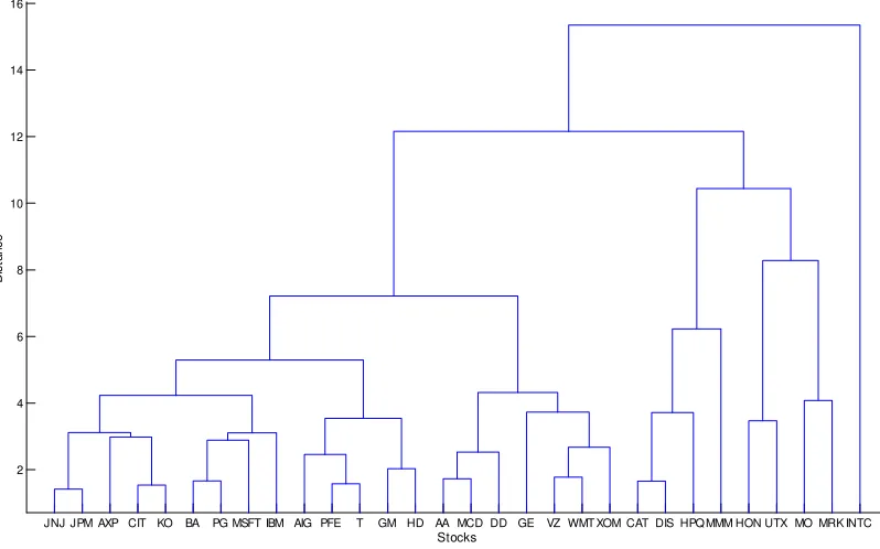
JNJ JPM AXP CIT KO BA PG MSFT IBM AIG PFE T GM HD AA MCD DD GE VZ WMT XOM CAT DIS HPQ MMM HON UTX MO MRK INTC 2

4 6 8 10 12 14 16

Stocks

D

ist

a

n

ce

Figure 1: Complete linkage dendrogram for DJIA stocks using the Mahalanobis-TGARCH distance

Wichern, 2007).

As we want to use a sensible number of groups, this dendrogram suggests three to …ve clusters. We decided to consider …ve clusters. One is composed of most …nancial, consumer goods and healthcare cor-porations, some technology corporations (IBM, Microsoft and AT&T) and Home Depot and Boeing. The second is composed of basic mate-rials and most services corporations and General Electric and Verizon. The third is composed of miscellaneous sector corporations (Caterpillar, Walt-Disney, Hewlett-Packard and 3M Co.). The fourth is composed of the industrial goods corporation Honeywell and the conglomerate cor-poration United Technologies. The …fth is composed of the consumer goods corporation Altria and the healthcare corporation Merck. The Inter-Tel corporation is not grouped.

MRK UTX HD PG INTC AA PFE JNJ MCD AIG GE KO CAT T VZ WMT DD MMM XOM AXP BA MSFT GM CIT JPM DIS IBM HON HPQ MO 40

60 80 100 120 140 160 180

D

ist

a

n

ce

Stocks

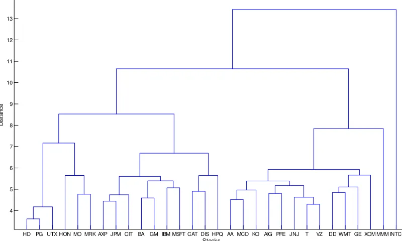
Figure 2: Complete linkage dendrogram for DJIA stocks using the LNP-based distance

second group is composed of technology (IBM, Microsoft and Hewlett-Packard), …nancial (American Express and JP Morgan Chase), industrial goods (Boeing, Citigroup and Honeywell), and consumer goods (Altria and General Motors) corporations. The third group is composed of miscellaneous sector corporations (Merck, United Technologies, Home Depot, Procter & Gamble and Inter-Tel).

HD PG UTX HON MO MRK AXP JPM CIT BA GM IBM MSFT CAT DIS HPQ AA MCD KO AIG PFE JNJ T VZ DD WMT GE XOM MMM INTC 4

5 6 7 8 9 10 11 12 13

Stocks

D

ist

a

n

ce

5

Multidimensional scaling

Multidimensional scaling is a multivariate statistical method that uses the information about the similarities (or dissimilarities) between the objects (in our case, time series) to construct a con…guration ofk points in the p-dimensional space. See, for instance, Everitt and Dunn (2001) and Johnson and Wichern (2007).

LetDbe the observedk k matrix of Euclidean distances. By mul-tidimensional scaling, the matrix D yields a k p con…guration matrix

T. The rows ofT are the coordinates of thek points in ap-dimensional representation of the observed dissimilarities (p < k). Thep-dimensional representation that best approximates the observed dissimilarity matrix is given by the p eigenvectors of T T0 _{corresponding to the p largest}

eigenvalues.

When the observed dissimilarity matrixD is not Euclidean, the ma-trix T T0 _{is not positive semi-de…nite. In such cases some of the}

eigen-values of T T0 _{will be negative. If, however, the sum of the positive}

eigenvalues of T T0 _{is approximately equal to the sum of all the}

eigenval-ues and the magnitude of the largest positive eigenvaleigenval-ues exceeds clearly that of the largest negative eigenvalue, the spatial con…guration of the observed dissimilarity matrix may still be advisable (Sibson, 1979).

As in the previous section, we will discuss separately the results of the three considered methods: the TGARCH, the LNP, and the combined TGARCH-LNP.

Firstly, table 4 shows the eigenvalues resulting from TGARCH dis-tances between stocks and the eigenvectors associated with the …rst two eigenvalues. Since D is non-Euclidean distance, some eigenvalues are negative. The …rst eigenvalue is equal to 54.0% of the sum of all the eigenvalues (583.5). The second eigenvalue is equal to 23.0% of the sum of all the eigenvalues. The sum of the …rst four positive eigenvalues (565.1) is almost equal to the sum of all the eigenvalues. The magnitude of the …rst two eigenvalues (315.1 and 134.1) exceed clearly the magni-tude of the largest negative eigenvalue (-37.2). The resulting solution ful…lls the trace and magnitude adequacy criterions of Sibson (1979).

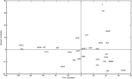
The size criterions of Mardia, Kent and Bibby (1979) suggest using the eigenvectors associated with the …rst two eigenvalues to represent the distances among stocks. Figure 4 shows the two-dimensional scaling map of the derived coordinate values. This plot can also help to identify the clusters.

-10 -8 -6 -4 -2 0 2 4 -4

-3 -2 -1 0 1 2 3 4 5

AA AIG

AXP BA

CAT

CIT

DD

DIS G E

G M HD HO N

HPQ

IBM

INTC

JNJ JPM

KO

MCD

MMM MO

MRK

MSF T

PFE PG

T UTX

VZ

W MT XO M

First coordinate

S

ec

ond

c

oor

d

inat

e

are clearly separated from each other and from the remainder indus-trial goods corporations. Conglomerate corporations (3M and United Technologies) are in di¤erent locations. Again, Inter-Tel corporation is a clear outlier.

This …rst coordinate seems to translate the distribution tail behav-ior. Stocks with estimated tail-thickness parameter close to 1 (INTC, MMM, MRK and MO) are in the negative region of the …rst coordinate, while those with estimated close to 1.5 are clustered at the positive region. This means that the higher probability of having extreme shocks is a …rst major factor for distinguishing the stocks.

Looking at the second coordinate, we notice that basic materials and services corporations have negative eigenvalues and tend to clus-ter together, and that most …nancial, technology, consumer goods and healthcare corporations appear to form a distinct group. Again, the two conglomerate corporations are very clearly separated from each other.

This second coordinate seems to incorporate the magnitude of the asymmetric shocks to volatility played by the -coe¢cient. This means that the asymmetry is a second major factor for distinguishing the stocks.

Secondly, we consider the LNP method. Figure 5 shows the corre-sponding scaling map of the DJIA stocks. The map tends to group the basic materials, the communications, and most healthcare, …nancial and services corporations in a distinct cluster and most technology, industrial goods and consumer goods corporations in another distinct cluster.

To better interpret the two principal coordinates of the LNP method, we have computed the smoothed log normalized periodograms for each of the 30DJIA squared return series. Figure 6 shows the corresponding plots.

The spectral function estimates are very diverse and the dissimilar-ities arise in the whole range of coordinates. The interpretation is very di¢cult. We notice that the …rst coordinate reveals a separate group at the left in which most corporations have an atypical spectral shape (PG, MRK, UTX, and HD). For these corporations, the spectra does not display a slowly decreasing long-term power, i.e., do not decrease regularly from the low to the higher frequencies. The second coordinate is even harder to interpret. We only highlight a clear separation of the communications corporationss (VZ and T) from the others.

-120 -100 -80 -60 -40 -20 0 20 40 60 80 -20

-10 0 10 20 30 40

AA AIG

AXP

BA CAT

CIT

DD DIS

G E G M

HD

HO N HPQ

IBM INTC

JNJ JPM

KO MCD

MMM MO

MRK

MSF T

PFE PG

T

UTX

VZ

W MT

XO M

First coordinate

S

ec

ond

c

oor

d

inat

e

-1 . 8 5 -1 . 8 0 -1 . 7 5 -1 . 7 0

5 0 0 1 0 0 0 1 5 0 0

AA

-1 . 9 5 -1 . 9 0 -1 . 8 5 -1 . 8 0 -1 . 7 5

5 0 0 1 0 0 0 1 5 0 0

AIG

-1 . 8 5 -1 . 8 0 -1 . 7 5 -1 . 7 0 -1 . 6 5 -1 . 6 0

5 0 0 1 0 0 0 1 5 0 0

AXP

-2 . 0 -1 . 9 -1 . 8 -1 . 7 -1 . 6 -1 . 5

5 0 0 1 0 0 0 1 5 0 0

BA

-1 . 9 0 -1 . 8 5 -1 . 8 0 -1 . 7 5 -1 . 7 0 -1 . 6 5 -1 . 6 0

5 0 0 1 0 0 0 1 5 0 0

CAT

-2 . 2 -2 . 0 -1 . 8 -1 . 6 -1 . 4

5 0 0 1 0 0 0 1 5 0 0

CIT

-1 . 9 5 -1 . 9 0 -1 . 8 5 -1 . 8 0 -1 . 7 5 -1 . 7 0

5 0 0 1 0 0 0 1 5 0 0

DD

-1 . 8 0 -1 . 7 8 -1 . 7 6 -1 . 7 4 -1 . 7 2 -1 . 7 0

5 0 0 1 0 0 0 1 5 0 0

DIS

-2 . 1 -2 . 0 -1 . 9 -1 . 8 -1 . 7 -1 . 6

5 0 0 1 0 0 0 1 5 0 0

GE

-1 . 8 5 -1 . 8 0 -1 . 7 5 -1 . 7 0 -1 . 6 5 -1 . 6 0

5 0 0 1 0 0 0 1 5 0 0

GM

-1 . 4 8 -1 . 4 6 -1 . 4 4 -1 . 4 2 -1 . 4 0

5 0 0 1 0 0 0 1 5 0 0

HD

-1 . 9 -1 . 8 -1 . 7 -1 . 6 -1 . 5

5 0 0 1 0 0 0 1 5 0 0

HON

-1 . 9 0 -1 . 8 5 -1 . 8 0 -1 . 7 5 -1 . 7 0 -1 . 6 5

5 0 0 1 0 0 0 1 5 0 0

HPQ

-1 . 9 0 -1 . 8 5 -1 . 8 0 -1 . 7 5 -1 . 7 0

5 0 0 1 0 0 0 1 5 0 0

IBM

-2 . 4 -2 . 2 -2 . 0 -1 . 8 -1 . 6

5 0 0 1 0 0 0 1 5 0 0

INTC

-1 . 8 0 -1 . 7 5 -1 . 7 0 -1 . 6 5 -1 . 6 0

5 0 0 1 0 0 0 1 5 0 0

J NJ

-2 . 2 -2 . 0 -1 . 8 -1 . 6 -1 . 4

5 0 0 1 0 0 0 1 5 0 0

J PM

-2 . 1 -2 . 0 -1 . 9 -1 . 8 -1 . 7 -1 . 6

5 0 0 1 0 0 0 1 5 0 0

KO

-2 . 0 -1 . 9 -1 . 8 -1 . 7 -1 . 6 -1 . 5

5 0 0 1 0 0 0 1 5 0 0

MCD

-1 . 9 0 -1 . 8 5 -1 . 8 0 -1 . 7 5 -1 . 7 0

5 0 0 1 0 0 0 1 5 0 0

MMM

-1 . 7 2 -1 . 6 8 -1 . 6 4 -1 . 6 0 -1 . 5 6

5 0 0 1 0 0 0 1 5 0 0

MO

-1 . 3 8 -1 . 3 7 -1 . 3 6 -1 . 3 5 -1 . 3 4 -1 . 3 3

5 0 0 1 0 0 0 1 5 0 0

MRK

-1 . 9 0 -1 . 8 5 -1 . 8 0 -1 . 7 5 -1 . 7 0 -1 . 6 5

5 0 0 1 0 0 0 1 5 0 0

MSFT

-2 . 0 -1 . 9 -1 . 8 -1 . 7 -1 . 6

5 0 0 1 0 0 0 1 5 0 0

PFE

-1 . 2 6 -1 . 2 4 -1 . 2 2 -1 . 2 0 -1 . 1 8

5 0 0 1 0 0 0 1 5 0 0

PG

-2 . 0 0 -1 . 9 5 -1 . 9 0 -1 . 8 5 -1 . 8 0 -1 . 7 5

5 0 0 1 0 0 0 1 5 0 0

T

-1 . 5 -1 . 4 -1 . 3 -1 . 2 -1 . 1

5 0 0 1 0 0 0 1 5 0 0

UTX

-2 . 0 -1 . 9 -1 . 8 -1 . 7

5 0 0 1 0 0 0 1 5 0 0

VZ

-2 . 0 0 -1 . 9 5 -1 . 9 0 -1 . 8 5 -1 . 8 0 -1 . 7 5

5 0 0 1 0 0 0 1 5 0 0

WMT

-2 . 0 -1 . 9 -1 . 8 -1 . 7

5 0 0 1 0 0 0 1 5 0 0

XOM

-8 -6 -4 -2 0 2 4 6 -6 -5 -4 -3 -2 -1 0 1 2 3 4 AA AIG AXP BA CAT CIT DD DIS G E G M HD HO N HPQ IBM INTC JNJ JPM KO MCD MMM MO MRK MSF T PFE PG T UTX VZ W MT XO M

First coordinate

S ec ond c oor d inat e

Figure 7: Two-dimensional scaling map of DJIA stocks using the com-bined LNP-TGARCH distance

is composed of most technology, …nancial and industrial good corpora-tions. The third is composed of most consumer goods corporations and a miscellaneous sector corporations. Again, corporations with null and negative shocks on volatility (3M Co. and Inter-Tel) are in distinct lo-cations and far from the other clusters.

The combined scaling map maintains the importance of the tail thick-ness for distinguishing the stocks (as we can see in the …rst map coordi-nate) and better clusters a central group.

6

Conclusions

In this paper, we introduced parametric and spectral-based distances for comparing and clustering multiple …nancial time series. Our method-ological contribution consists essentially in adding the internal stochastic dynamic features to the comparison and in providing a combined dis-tance that takes into account both the estimated model parameters and the spectral behavior of stocks’ volatility.

multidimensional scaling techniques, we found that all considered meth-ods (LNP, TGARCH, and combined TGARCH-LNP) are able to get meaningful corporate sector clusters. We found homogenous clusters of stocks with respect to the basic materials, services, healthcare, …nancial, communications and technology corporate sectors, and we found hetero-geneous clusters of stocks with respect to the conglomerates, industrial goods, and consumer goods corporate sectors.

The TGARCH method tends to collect most …nancial, technology, consumer goods, and healthcare corporations into a cluster and basic materials and most services corporations into another one. The LNP method tends to group most technology and industrial good corporations into a cluster, and basic materials, communications and most healthcare corporations into another one. The combined TGARCH-LNP method tends to group most …nancial and technology corporations into a cluster, basic materials, communications and most healthcare corporations into another one, and most consumer goods into a third one.

In all cases, the thickness of the tail distribution plays an important discriminating role. This suggests that a higher probability of displaying extreme events seems to be an important factor in the classi…cation of stocks. In the TGARCH method, the asymmetry parameter also plays an important role. This suggests that a di¤erent response to good and bad news is an important stock volatility discriminating factor.

The TGARCH and LNP methods led to somehow similar cluster solutions, which is very reassuring. The introduction of the combined TGARCH-LNP method allows for a potentially more reliable di¤erenti-ation between the series, as it uses more informdi¤erenti-ation about the dynamic features of the stock returns and volatilities.

Acknowledgment: The authors are grateful to several anonymous

referees for helpful comments and suggestions that vastly improved this article. They also thank the comments of participants in the COMP-STAT’2008 International Conference on Statistical Computing. This research was supported by a grant from the Fundação para a Ciência e a Tecnologia (FEDER/POCI 2010).

References

[1] Bekaert, G. and Wu, G. (2000). "Asymmetric volatility and risk in equity markets", Review of Financial Studies, 13, 1-42.

[2] Bollerselev, T. Chou, R. and Kroner, K. (1992). “ARCH modeling in Finance”, Journal of Econometrics, 52, 5-59.

cross-correlation in a set of stocks", Quantitative Finance, 1, 96-104.

[4] Bonanno, G., Caldarelli, G., Lillo, F., Miccieché, S., Vandewalle N. and Mantegna, R. (2004). "Networks of equities in …nancial mar-kets", European Physical Journal B, 38, 363-371.

[5] Caiado, J., Crato, N. and Peña, D. (2006). "A periodogram-based metric for time series classi…cation", Computational Statistics & Data Analysis, 50, 2668-2684.

[6] Caiado, J., Crato, N. and Peña, D. (2009). "Comparison of time series with unequal length in the frequency domain", Communica-tions in Statistics - Simulation and Computation, 38, 527-540. [7] Engle, R. and Kroner. K. (1995). "Multivariate simultaneous

gen-eralized ARCH", Econometric Theory, 11, 122-150.

[8] Everitt, B. and Dunn, G. (2001).Applied Multivariate Data Analy-sis, 2th Ed., Hodder Arnold, London.

[9] Everitt, B., Landau, S. and Leese, M. (2001).Cluster Analysis, 4th Ed., Edward Arnold, London.

[10] Glosten, L. Jagannathan, R. and Runkle, D. (1993). "On the rela-tion between the expected value and the volatility of the nominal excess return on stocks", The Journal of Finance, 48, 1779-1801. [11] Gordon, A. (1996). "Hierarchical classi…cation", in Clustering and

Classi…cation, P. Arabie, L. J. Hubert and G. De Soete (Eds.),

World Scienti…c Publ., River Edge, NJ.

[12] Johnson, R. and Wichern, D. (2007). Applied Multivariate Statisti-cal Analysis. 6th Ed., Prentice-Hall.

[13] Kroner, K. and Ng, V. (1998). “Modeling asymmetric comovements of asset returns”, Review of Financial Studies, 11, 817-844.

[14] Mantegna, R. N. (1999). "Hierarchical structure in …nancial mar-kets", The European Physical Journal B, 11, 193-197.

[15] Mardia, K., Kent, J., and Bibby, J. (1979). Multivariate Analysis, Academic Press, London.

[16] McLeod, A. and Li, W. (1983). "Diagnostic checking ARMA time series models using squared-residual autocorrelations", Journal of Time Series Analysis, 4, 269-273.

[17] Nelson, D. (1991). "Conditional heteroskedasticity in asset returns: a new approach", Econometrica, 59, 347-370.

[18] Sibson, R. (1979). "Studies in the robustness of multidimensional scaling: Perturbational analysis of classical scaling",Journal of the Royal Statistical Society B, 41, 217-229.

[19] Tsay, R. (2005),Analysis of Financial Time Series, 2nd Ed., Wiley, New Jersey.

of Economic Dynamics and Control, 18, 931-944.

[21] Zivot, E. and Wang, J. (2003).Modeling Financial Time Series with

Table 1: Stocks used to compute the Dow Jones Industrial Average (DJIA) Index

Stock Code Sector Stock Code Sector

Alcoa Inc. AA Basic materials Johnson & Johnson JNJ Healthcare American Int. Group AIG Financial JP Morgan Chase JPM Financial

American Express AXP Financial Coca-Cola KO Consumer goods Boeing Co. BA Industrial goods McDonalds MCD Services

Caterpillar Inc. CAT Financial 3M Co. MMM Conglomerates Citigroup Inc. CIT Industrial goods Altria Group MO Consumer goods El Dupont DD Basic materials Merck & Co. MRK Healthcare Walt Disney DIS Services Microsoft Corp. MSFT Technology General Electric GE Industrial goods P…zer Inc. PFE Healthcare General Motors GM Consumer goods Procter & Gamble PG Consumer goods Home Depot HD Services AT&T Inc. T Technology Honeywell HON Industrial goods United Technol. UTX Conglomerates Hewlett-Packard HPQ Technology Verizon Communic. VZ Technology Int. Bus. Machines IBM Technology Walt-Mart Stores WMT Services

Table 2: Summary statistics for Dow Jones Industrial Average (DJIA) stock returns

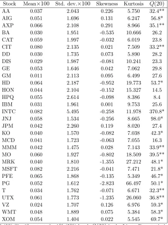
Stock Mean 100 Std. dev. 100 Skewness Kurtosis Q(20)

AA 0.037 2.043 0.226 5.750 32.4** AIG 0.051 1.696 0.131 6.247 56.8* AXP 0.066 2.108 0.291 8.966 35.1** BA 0.030 1.951 -0.535 10.666 26.2 CAT 0.059 1.997 -0.032 6.019 23.8 CIT 0.080 2.135 0.021 7.509 33.2** DD 0.030 1.735 0.073 5.890 28.2 DIS 0.029 1.987 -0.081 10.241 23.3 GE 0.053 1.646 0.042 7.062 29.8 GM 0.011 2.113 0.095 6.499 27.6 HD 0.064 2.187 -0.952 19.773 53.7* HON 0.044 2.104 -0.152 15.327 14.5 HPQ 0.055 2.614 -0.098 8.386 8.4 IBM 0.031 1.961 0.001 9.753 25.6 INTC 0.082 5.495 -0.258 11.978 370.8* JNJ 0.058 1.534 -0.256 8.665 98.0* JPM 0.042 2.260 0.119 8.020 27.4 KO 0.040 1.570 -0.082 7.038 42.3* MCD 0.041 1.723 -0.063 7.055 16.3 MMM 0.042 1.475 0.028 7.143 33.9** MO 0.060 1.927 -0.802 18.509 39.5** MRK 0.040 1.810 -1.355 27.212 48.1* MSFT 0.082 2.216 -0.041 7.471 21.8* PFE 0.065 1.868 -0.135 5.349 46.7* PG 0.052 1.612 -2.823 66.497 50.1* T 0.034 1.762 -0.071 6.671 32.3** UTX 0.061 1.773 -1.235 26.060 36.8** VZ 0.024 1.707 0.126 6.976 59.3* WMT 0.048 1.889 0.075 5.384 58.3* XOM 0.054 1.404 0.022 5.545 69.7*

Table 3: Estimated TGARCH(1,1) models assuming GED innovations for DJIA stock returns

Table 4: Eigenvalues and eigenvectors resulting from TGARCH dis-tances between DJIA stocks