About the Mean Difference of the Inverse Normal Distribution

http://dx.doi.org/10.4236/am.2016.714130

About the Mean Difference of the Inverse

Normal Distribution

Giovanni Girone, Angela Maria D’Uggento

Department of Economics and Mathematical Methods, University of Bari Aldo Moro, Bari, Italy

Received 9 June 2016; accepted 15 August 2016; published 18 August 2016

Copyright © 2016 by authors and Scientific Research Publishing Inc.

This work is licensed under the Creative Commons Attribution International License (CC BY). http://creativecommons.org/licenses/by/4.0/

Abstract

The calculation of the mean difference for the inverse normal distribution can be obtained by a transformation of variable or a hard integration by parts. This paper shows a simpler formula of the mean difference of the inverse normal distribution that highlights the role of the two parame-ters on the mean difference of the model. It makes it easier to study the relation of the mean dif-ference with the other indexes of variability for the inverse normal distribution.

Keywords

Mean Difference, Inverse Normal Distribution

1. Introduction

variability do. The above mentioned studies do not treat the formula of the mean difference for the Wald inverse normal distribution. The aim of this paper is to partly fill in this gap.

2. The Inverse Normal Distribution

The density function of the inverse normal distribution is

( )

( )

2 2 2

3e , 0 , 0, 0.

2π

x x

f x x

x

λ µ µ

λ − − _{µ λ}

= < < ∞ > > (1)

The cumulative distribution function of the inverse normal distribution is

( )

( 2) 2

2 3

0 ₂π e d , 0.

u x

u

F x u x

u

λ µ µ

λ − −

=

_∫

> (2)

The cumulative distribution function can also be written as

( )

2

1 e 1 , 0,

x x

F x x

x x

λ µ

λ λ

µ µ

     

= Φ_{ } − _+ Φ_{ } + _ >

   

    (3)

in which

( )

2

2

e d 2π

u x

x u

−

−∞

Φ =

_∫

(4)

is the cumulative distribution function of the standard normal distribution. The mean and the variance of this distribution are, respectively,

( )

,

E X =µ (5)

and

( )

2

Var X µ

λ

= . (6)

3. Calculation Procedure for the Mean Difference of a Continuous Distribution

A continuous distribution is characterized by the density function

( )

0,

f x = − ∞ < <x a, (7)

( )

0, ,

f x > a< <x b (8)

( )

0, ,

f x = b< < ∞x (9)

or by the cumulative distribution function

( )

0, ,

F x = − ∞ < <x a (10)

( )

x

( )

d , a

F x =

∫

f x x a< <x b, (11)

( )

1, .

F x = b< < ∞x (12)

Moreover, the first incomplete moment is

( )

1 0, ,

F x = − ∞ < <x a (13)

( )

( )

1 d , ,

x

F x =

∫

_−∞xf x x a< <x b (14)

( )

1 , .

In the previous formulas, a can be also equal to −∞ and b equal to +∞.

To compute the mean difference of a continuous distribution between the two values x and y of the same random variable, one of the following four formulas can be used.

The direct formula is

(

) ( ) ( )

2 b x d d ,

a a x y f x f y y x

∆ =

_{∫ ∫}

− (16)

the formula based on the density function and the cumulative distribution function is

( )

( )

2 b 2 1 d ,

ax F x f x x

∆ =

_∫

_ − _ (17)

another option is the formula based on the density function, the cumulative distribution function and the first incomplete moment is

( )

1

( ) ( )

2 b d ,

a x F x F x f x x

∆ =

_∫

_ − _ (18)

and, finally, the formula based solely on the cumulative distribution function is

( )

( )

2 b 1 d .

aF x F x x

∆ =

_∫

_ − _ (19)

The previous four formulas are completely equivalent, although, depending on the models whose mean difference has to be calculated, some of them are easier to apply if compared to the others.

4. Calculation Procedure for the Mean Difference of the Inverse Normal

Distribution

If we consider the formula based on the cumulative distribution function, the mean difference is

( )

( )

0

2 ∞F x 1 F x d .x

∆ =

_∫

_ − _ (20)

Replacing the cumulative distribution function of the inverse normal distribution, leads to

(

)

(

)

2 2

0 1

1 e d

2 2 2

x x

Erf Erfc x

x x

λ µ

λ µ λ µ

µ µ

∞ _   −   +  _

 

∆ = _ −_  +  _{ }

   

   

 

 

∫

, (21)

in which there are the error function

( )

2

0 2

e d π

x _t

Erf x =

∫

− t (22)

and the complementary error function

( )

1

( )

Erfc x = −Erf x (23)

The Error function is encountered in integrating the normal distribution, which is a normalized form of the Gaussian function. Then, introducing the transformation of the variable

X V

µ

= (24)

and denoting

φ= λ µ (25)

this formula is obtained

(

)

2

(

)

2 2

0

1 1

1

1 e d

2 2 2

v v

Erf Erfc v

v v

φ

φ φ

µ ∞    −   +  

∆ = _ −_  +  _{ }

   

 

 

∫

(26)

The function to be integrated, unless the constant 1/2, has the structure 1−h v

( )

,φ 2. Introducing the transformation of variable

(

)

1 , ,

Z = −h V φ (27)

after heavy but direct calculations, the following expression is achieved ( )₁2 2

₍

₎

2

0

1 e

2

4 d .

2π

z

z _Erf z

u z

z z

φ _φ

φ µ

− −

∞

−

 

 

 

∆ = −

_∫

(28)

For simplicity, in the above formula the following transformation of the variable should be introduced

(

1

)

2

Z Y

Z φ −

= (29)

which, after further heavy but direct calculations, leads to

( )

2

0 2 2

8e

d ,

π 2

y

yErf y y y

µ

φ

− ∞

∆ =

+

∫

(30)

in which the integral exists for any value of μ and for φ > 0. The analytical value of Δ is not known but its value can be easily numerically calculated.

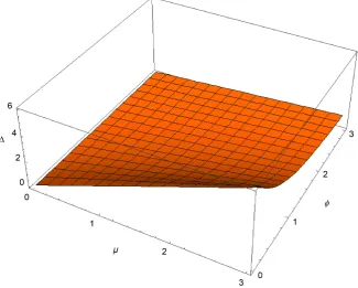
[image:4.595.152.478.429.690.2]

The obtained expression is the simplest formula enabling to compute the mean difference of the inverse nor-mal distribution. The above formula clearly highlights the role of the two parameters: one, μ, is a multiplicative factor and the other one, ϕ, is part of the function to be integrated.

Figure 1 shows the trend of the mean difference of the inverse normal distribution as function of the parame-ters μ and ϕ. It can be observed that Δ increases with the parameter μ and decreases as the parameter ϕ increases. Through a transformation of variable or an integration by parts, several other equivalent formulas can be ob-tained, all of them needing an integration. Some of them are shown in the Appendix.

5. Conclusive Remarks

In this paper, a simple formula of the mean difference of the inverse normal distribution is achieved. The for-mula is simpler than those obtainable by a transformation of variable or an integration by parts of the same. Even if the formula contains an integration to be computed, it is undoubtedly easy to calculate and allows to highlight the role of the two parameters on the mean difference of the model. It makes it easier to study the rela-tion of the mean difference with the other indexes of variability for the inverse normal distriburela-tion.

References

[1] Norman, J.L., Samuel, K. and Narayanaswamy, B. (1994/1995) Continuous Univariate Distributions. Wiley, New York, Vol. 1, 1994; Vol. 2, 1995.

[2] Jagdish, P.K., Kapadia, C.H. and Owen, D.B. (1976) Handbook of Statistical Distributions. Dekker, New York. [3] Girone, G. and Mazzitelli, D. (2007) La differenza media nei principali modelli distributivi continui. In: Annali del

Dipartimento di Scienze Statistiche “Carlo Cecchi”, dell’Università degli Studi di Bari, Vol. 7, tomo I, Cacucci Editore, Bari, 45-61.

[4] Girone, G. and Viola, D. (2009) La differenza media della distribuzione di Dagum. Annali del Dipartimento di Scienze statistiche “Carlo Cecchi” dell’Università degli Studi di Bari, 8, 101-106.

[5] Girone, G., Massari, A. and Mazzitelli, D. (2015) More on the Mean Difference of Continuous Distribution Models.

Proceedings of the SIS Conference “Statistics and Demography: The Legacy of Corrado Gini”, Treviso, 9-11 September 2015, 1-8. http://meetings.sis-statistica.org/index.php/ginilegacy/SIS2015/paper/view/3675/771

[6] Girone, G. and Massari, A. (2015) La differenza media della variabile F di Snedecor, in Studi in ricordo di Carlo Cecchi. Università degli Studi di Bari Aldo Moro, Bari.

[7] Girone, G., Manca, F. and D’Uggento, A.M. (2015) The Mean Difference of Discrete Distribution Models.

Proceedings of the SIS Conference “Statistics and Demography: The Legacy of Corrado Gini”, Treviso, 9-11 Sep- tember 2015, 1-6.http://meetings.sis-statistica.org/index.php/ginilegacy/SIS2015/paper/view/3532/740

Appendix:

Alternative Formulas for Calculating Δ for the Inverse Normal

Distribution

( )

2

0 2 2

8 e d π 2 y yErf y y y µ φ − ∞ ∆ = +

∫

(31)

(

)

2 2

2 2 2

2

8 e 2

d π y Erf y y φ φ

µ − φ

∞ −

∆ =

_∫

(32)

( )

(

)

2 2

3 2

0 2 2

4 2 d 2 Erf y y y µφ µ φ ∞ ∆ = − +

∫

(33)

(

)

2

2 2 2

2 2 2 2

4 2 2 d 2 Erf y y y y φ µφ φ µ φ ∞ − ∆ = − −

∫

(34)

(

)

2 2 2

2 2 2

2 0

8 e 2

4 e d

π y

Erf y

y

φ

φ µ φ

µ

−

∞ +

∆ = −

_∫

(35)

( )

2 2

2 4

2

2 2 2

8 e

4 e d

π 2 y yErf y y y φ φ φ µ µ φ − ∞ ∆ = − −

∫

(36)

(

)

( )

(

)

2 ₂

2 2

3 2

0 2 2

4 e 0, 2 4 e

d

π _{π 2}

y

BesselK yErf y

y y

φ

µ φ _µ

φ

− ∞

∆ = −

+

∫

(37)

(

)

2 2

(

)

2 2 2 2

2 2

2 2

4 e 2

4 e 0, 2

d π π y Erf y BesselK y y φ φ φ

µ µ φ

µ φ ∞ − + −

∆ = −

_∫

(38)

(

)

2 2 2

2 _{2 2 2 2}

2

0 1

2 , 0, 4 _{16 6e 2}

2

4 e d

π π

y

HypergeometricU _{y Erf y}

y

φ φ

µ φ _{µ φ}

µ − ∞     +  

∆ = + −

_∫

(39)

( )

2 2 2

2

4 2 2

2

2 1

2 , 0, 4

16 e 2

2

4 e d

π π

y

HypergeometricU

y y Erf y

y

φ φ

φ

µ φ _{µ φ}

µ ∞ −

 

  ₋

 

∆ = + −

_∫

(40)

( )

2 _{2 2} 2

0

1

4 , 0, 4

16 e 2 2

d

π π

y HypergeometricU

y y Erf y

y

µ φ

µ − φ

∞

₋ 

 

+ _{ }

∆ =

_∫

− (41)

(

)

2 2 2

2 2 2 2

2

1

4 , 0, 4

16 e 2

2 d

π π

y _{HypergeometricU}

y Erf y

y

φ

φ

µ φ

µ − φ

∞

₋ 

 

−

 

∆ =

_∫

− (42)

( )

₍

₎

2 2 2 2 2 0

8 e 2 1

2 e 0, 2

2

d

π π

y y

y ArcSinh Erf y

BesselK y

φ

µ _{µ φ}

φ − ∞    −  _{ }   _{ }

∆ =

_∫

− (43)

Submit or recommend next manuscript to SCIRP and we will provide best service for you:

Accepting pre-submission inquiries through Email, Facebook, LinkedIn, Twitter, etc. A wide selection of journals (inclusive of 9 subjects, more than 200 journals) Providing 24-hour high-quality service

User-friendly online submission system Fair and swift peer-review system

Efficient typesetting and proofreading procedure

Display of the result of downloads and visits, as well as the number of cited articles Maximum dissemination of your research work