©IJRASET: All Rights are Reserved
292
PID Controller Tuning and Its Case Study
Smitha A B1, Sachin C N Shetty 2, Bianca Baby3 1
(M.Tech in VLSI & Embedded Systems, Sahyadri college of Engineering and Management, India) 2,3
(Assistant Professor, Dept. Electronics and Communication Department, Sahyadri college of Engineering and Management, India)
Abstract This paper has been like to presents the Comparative study of Proportional (P), Proportional Integral (PI), and Proportional Integral Derivative (PID) controllers. The PID controller is one of the most commonly used dynamic control technique. Over 85% of all low level controllers are of the PID family. The purpose of this report is to provide a brief overview and advantage of using the PID controller rather than P and PI controllers. Different tuning methods include Manual Tuning Method, Ziegler-Nichols Method are used to get the stable output response. The parameters must be identified and tuned for the good performance Manual Tuning Method, Ziegler-Nichols Method
Keywords Control system, Parameter, PID controller, Ziegler-Nichols Method
I. INTRODUCTION
The PID controller calculation includes three basic behavior, the Proportional, the Integral and the Derivative. These three behavior form the PID calculation. The proportional parameter determines the reaction to the current error, the integral parameter determines the reaction based on the sum of past errors and the derivative value determines the reaction based on the rate at which the error has been changing i.e. future error. The total sum of these three parameters is used to adjust the plant (object to be controlled) via a control element such as the position of a control valve or the temperature of a heating element. By tuning these three constants in the PID control system, the controller can provide control over the specific process requirements. The response of the controller can be described by using speed, accuracy and stability of the controller.
Some applications may use only one or two of the parameters to provide the appropriate control of the system. This is done by setting the gain of undesired control gain to zero. For example a PID controller can be used as PI, PD, P or I controller by setting the undesired control gain to zero. The three parameters of a PID controller must be tuned properly by using different tuning methods to obtain a desired closed loop system performance. In spite of their simplicity, they can be used to solve many complex calculations, especially when combined with different functional blocks, filters, selectors etc
II. PID ALGORITHM
A PID controller is a simple three-term controller.
The letters P, I and D stand for P – Proportional, I – Integral, D - Derivative The transfer function of the basic form of PID controller is
C(s) = KP+KI/S+KDS
= KDS2 +KPS +KIS
Where KP = Proportional gain, KI = Integral gain and KD = Derivative gain.
Designing and tuning a Proportional Integral Derivative (PID) controller appears to be conceptually impulsive, but it is difficult in practice, if multiple objectives such as short transient response and high stability are to be achieved. PID controller has the good control dynamics including zero steady state error, short rise time, no oscillations and higher stability. The necessity of using a derivative gain component in addition to the PI controller is to remove the overshoot and the oscillations occurring in the output response of the system. The main advantages of the PID controller is that it can be used with higher order processes including more than single energy storage.
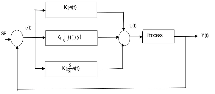
A typical structure of a PID control system is shown in Fig 1. The error signal e(t) is used to create the proportional, integral, and derivative actions, with the resulting signals weighted and added with the set point (SP) signal to form the control signal U(t)
©IJRASET: All Rights are Reserved
293
applied to the process model. Here the controller is used in a closed-loop unity feedback system. The variable e denotes the trailing error, which is sent to the PID controller. The control signal U(t) from the controller to the process is equal to the proportional gain (KP) times the magnitude of the error, the integral gain (KI) times the integral of the error and the derivative gain (KD) times thederivative of the error.
[image:3.612.115.476.196.354.2]Mathematically it is given as U(t)=KPe(t)+KI∫e(t)dt+KDde(t)/dt
Fig 1: Block diagram of PID controller
Here the Set Point (SP) is the value at which the user is trying to control the Process Variable (PV). The Process Variable is the parameter being controlled.
Proportional term, called as Gain, makes a change to the output that is proportional to the current error value. The bigger the error signal (PV-SP), bigger the correction that will be made to handle the variable. Big gains can cause a system to become unstable. Low gains can cause the system to respond too slowly to system disturbances. The Integral, or Reset Term, collects the instantaneous error value over a defined period of time and provides corrections based on this collected error. The amount of correction is based on the Integral value. When used in coincidence with the Gain factor, the Integral value helps to drive toward the set point, removes steady-state error. Since the Integral value is based on past error values, it can cause overshoot of the present value. The rate of change of the error signal is the basis of the Derivative (or Rate) factor. The Derivative factor tends to decrease the rate of change of the process variable. This behavior feels to reduce the chances of overshoot due to the Integral factor.
In PID controller, the relation between PID parameters and the system response specifications is clear. Each part has its certain function as follows:
A. Proportion can increase the response speed and control accuracy of the system. Larger KP can lead to faster response speed and
higher control accuracy. But if KP is too big, the overshoot will be large and the system will tend to be instable. Meanwhile, if
KP is too small, the control accuracy will be decreased and the regulating time will be prolonged. The static and dynamic
performance will be deteriorated.
B. Integration is used to eliminate the steady-state error of the system. With bigger KI, the steady-state error can be eliminated
faster. But if KI is too big, there will be integral saturation at the beginning of the control process and the overshoot will be
large. On the other hand, if KI is too small, the steady-state error will be very difficult to be eliminated and the control accuracy
will be bad.
C. Differentiation can improve the dynamic performance of the system. It can prevent and predict the change of the error in any direction. But if KD is too big, the response process will brake early, the regulating time will be prolonged and the
anti-interference capability of the system will be bad.
The digital PID controller can be described by the following difference equation
∑
SP
KPe(t)
Kt∫0 ( )
KD e(t)
∑
e(t)
Process
U(t)
©IJRASET: All Rights are Reserved
294
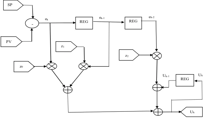
u(k)=u(k-1)+z0e(k)+z1e(k-1)+z2e(k-2)Where the coefficients z0, z1, and z2 are evaluated by the expressions:
z0 = KC(1+TD/TS)
z1 = -KC(1+2TD/TS-TS/TI)
z2 = KCTD/TS
The KC, TI and TD, are PID parameters for tuning, and TS is the sampling period in seconds. There are several methods for
evaluating the PID parameters, generally called PID tuning methods. When controlling time-invariant processes, the PID parameters can be constants and evaluated off-line, so, the PID architecture may use fixed values for the z0, z1 and z2 coefficients.
Otherwise, for time-variant processes there is a need to update those parameters; in this case the PID architecture has KC, TI and TD
as parameters that can be automatically updated during runtime by auto-tuning algorithms.
[image:4.612.125.483.270.476.2]Fig 2: Architecture of PID controller
Figure 2 shows a simple PID architecture with the z0, z1 and z2 coefficients. This architecture uses three adders, three multipliers
and three registers. The arithmetic operations may have saturation behavior so that whenever the magnitude of the result of an operation is not represented by the output representation, the result outputted is the largest or the smallest represented value. A complete implementation of the PID controller with auto-tuning requires a component responsible for the auto-tuning algorithm, whose complexity depends on the auto-tuning algorithm used. The auto-tuning feature is required in most control systems for mobile robotics due to the changes that may occur in the environment and system. Those modifications usually need the retuning of parameters to still have a stable control system with acceptable performance criteria.
III. PID CONTROLLER PARAMETER AND IDENTIFICATION
Problem of identification of PID controller arises when parameters of an existing controller have to be tuned. Controller parameters have to be manually tuned if they are changed with time or because process parameters have changed so the controller does not perform satisfactory anymore.
SP
PV
z0
z1
ek ek-1
z2
REG
Uk
REG
REG
-
ek-2
Uk
©IJRASET: All Rights are Reserved
295
Parameter Speed of Response stability accuracy
Increase KP Increases Drops Improves
Increase KI Decreases Drops Improves
Increase KD Increases Improves No impact
Table 1 Rules for tuning PID controller parameters
Identification can be performed experimentally using a certain type of reference signal on the controller input i.e. y(t) and measuring response on the controller output U(t).
Identification of the controller Proportional gain KP
[image:5.612.61.254.245.486.2]
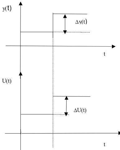
Fig 3.P controller response on step input
Proportional gain of the controller can be measured form transfer function of proportional channel of the controller. In order to that one should disconnect derivative and integral channel, or, if that is not possible one should set TD on zero and TI on very large value.
In that way the PID controller is reduced to P controller only. From the Fig 3 the response of such P controller it is possible to compute the proportional gain of the controller.
KP = ∆u/∆y
Identification of PID controller integral time constant TI
Integral time constant of the controller can be determined from the PI controller response by setting TD to zero. From the response
given in Fig 4 the integral time constant is determined as TI = KP(∆y/∆u)∆t
∆y(t)
∆U(t)
y(t)
U(t)
t
©IJRASET: All Rights are Reserved
296
[image:6.612.64.259.106.333.2]
Fig 4. PI controller response on step input
Identification of PID controller derivative time constant TD
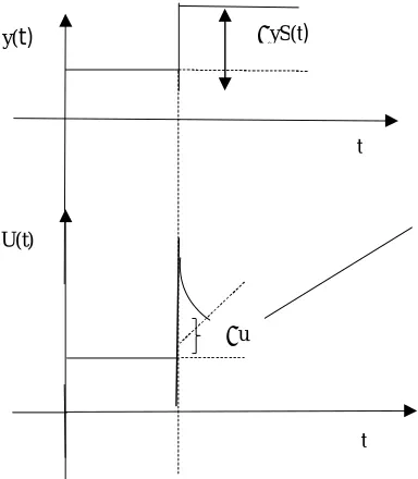
Fig 5. PD controller response on ramp input
Derivative time constant of the controller is determined from PD controller response on ramp input. Integral channel is disconnected or time constant TI is set to very large value. If responses of P and PD controller on ramp signal e(t) = A*t are compared, it can be
seen that response for P controller is given as: UP(t) = KPe(t)=KPA*t
The only difference in response is that PD controller gives value of control signal TD seconds before P controller. From the response
on the ramp input shown in Fig 5 it is possible to measure time constant TD.
Identification of PID controller topology
In order to identify PID controller topology it should work with all modes active. Then from the step response of PID controller shown in Fig 6 can be determined PID controller topology.
∆y(t)
∆U(t)
y(t)
U(t)
t
t
∆t
y(t)
U(t)
t
t A
1
©IJRASET: All Rights are Reserved
[image:7.612.64.256.106.326.2]297
Fig 6. Step response of PID controllerThe structure of the controller can be determined from the ratio ∆u/∆y. If ∆u/∆y = KP then structure of the controller is parallel and
if ∆u/∆y = KP(1+TD/TI) then structure of the controller is serial.
IV. LOOP TUNING
Tuning a control loop is arranging the control parameters to their optimum values in order to obtain desired control response. At this instant, stability is the main factor, but beyond that, different systems leads to different behaviors and requirements and these might not be compatible with each other. Theoretically, PID tuning seems completely easy, consisting of only 3 parameters, but, practically; it is a difficult problem because the complex criteria at the PID limit should be satisfied. PID tuning is mostly an abstractive concept but existence of many objectives to be met such as short transient, high stability makes this process harder. For example sometimes, systems might have nonlinearity problem which means that while the parameters works properly for full load conditions, they might not work as effective for no load conditions. Also, if the PID parameters are chosen wrong, control process input might be unstable, with or without oscillation; output diverges until it reaches to saturation or mechanical breakage. For a system to operate properly, the output should be stable, and the process should not oscillate in any condition of set point or disturbance.
In today’s control industrial applications, PID is used over 95% of the control loops. Actually if there is control, there is PID, in analog or digital forms. In order to achieve optimum solutions KP, KI and KD gains are arranged according to the system
characteristics. There are many tuning methods, but most common methods are as follows:
A. Manual Tuning Method
Manual tuning is achieved by arranging the parameters according to the system response. Until the desired system response is obtained KI, KP and KD are changed by observing system behavior.
Example (for no system oscillation): First lower the derivative and integral value to 0 and raise the proportional value 100. Then increase the integral value to 100 and slowly lower the integral value and observe the system’s response. Since the system will be maintained around set point, change set point and verify if system corrects in an acceptable amount of time. If not acceptable or for a quick response, continue lowering the integral value. If the system begins to oscillate again, record the integral value and raise value to 100. After raising the integral value to 100, return to the proportional value and raise this value until oscillation ceases. Finally, lower the proportional value back to 100 and then lower the integral value slowly to a value that is 10% to 20% higher than the recorded value when oscillation started. Although manual tuning method seems simple it requires a lot of time and experience.
∆yS(t)
y(t)
U(t)
t
t
©IJRASET: All Rights are Reserved
298
B. Ziegler-Nichols MethodZiegler-Nichols Method is one of the most effective methods that increase the usage of PID controllers. Firstly, it is checked that whether the desired proportional control gain is positive or negative. For this, step input is manually increased a little, if the steady state output increases, the proportional control gain is positive, otherwise; it is negative. Then, KI and KD are set to zero and only KP
value is increased until it creates a periodic oscillation at the output response. This critical KP value is attained to be ultimate gain,
KC and the period where the oscillation occurs is named as PC “ultimate period. As a result, the whole process depends on two
variables and the other control parameters are calculated according to the table given below.
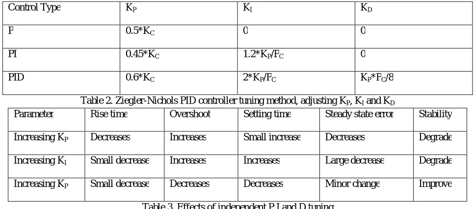
Control Type KP KI KD
P 0.5*KC 0 0
PI 0.45*KC 1.2*KP/PC 0
[image:8.612.64.547.187.400.2]PID 0.6*KC 2*KP/PC KP*PC/8
Table 2. Ziegler-Nichols PID controller tuning method, adjusting KP, KI and KD
Parameter Rise time Overshoot Setting time Steady state error Stability
Increasing KP Decreases Increases Small increase Decreases Degrade
Increasing KI Small decrease Increases Increases Large decrease Degrade
Increasing KP Small decrease Decreases Decreases Minor change Improve
Table 3. Effects of independent P I and D tuning
The PID parameters affect the system dynamic. Four major characteristics of the closed-loop step response are evaluated:
1) Rise time: - The time it takes for the control system output y to rise beyond 90% of the desired level for the first time. 2) Overshoot: - How much the peak level is higher than the steady state, normalized against the steady state.
3) Settling time: - The time it takes for the system to converge to its steady state.
4) Steady-state error: - The difference between the steady-state output and the desired output.
V. CONCLUSION
PID is a simple entity and broadly used in many of the industrial applications. PID controller has developed response after tuned properly. Various tuning methods can be proposed and used for the tuning of PID controller. The best values of PID constants are preferable for smooth control action. By tuning the three constants in the PID algorithm, the controller can provide control action fashioned for unique process requirements. The response of the controller can be represented in terms of rise time, overshoot, settling time, degree of oscillation, steady state error. Some activities may require using only one or two of the parameters to provide the better control of the system. This is achieved by setting the gain of undesired control outputs to zero. A PID controller will be called a PI, PD, P or I controller in the absence of the respective control actions. PI controllers are particularly common, since derivative action is very delicate to quantitative analysis of noise, and the absence of an integral value may protect the system from reaching its target value due to control action.
REFERENCES
[1] Shumit Saha, Md. Jahiruzzaman, Chandan Saha, Md. Rubel Hosen, Atiq Mahmud “Implementation of Modified Type-C PID Control System” 2nd Int'l Conf. on Electrical Engineering and Information & Communication Technology (ICEEICT) 2015 Iahangirnagar University, Dhaka-I 342, Bangladesh, 21-23 May 2015
[2] A. Trimeche, A. Sakly, A. Mtibaa, and M. Benrejeb, "PID control implementation using FPGA technology," 3'd International Conference on Design and Test Workshop, pp. 1-4,2008.
[3] L. Qu, Y. Huang, L. Ling, "Design and implementation of intelligent PID controller based on FPGA," IEEE 41h International Conference on Natural Computation, pp. 511-515,2008.
©IJRASET: All Rights are Reserved
299
Cybernetics, pp. 2577-2583, 2006.
[5] H. D. Maheshappa, R. D. Samuel, A. Prakashan, “Digital PID controller for speed control of DC motors”, IETE Technical Review Journal, V6, N3, PP171!176, India 1989