A Framework to Process Iceberg Queries using Set intersection and Set Difference Operations

A Framework to Process Iceberg Queries using

Set-intersection and Set-Difference Operations

Ch.Chaitanya Bharathi

M.Tech.(SE) Dept.of CSE Kakatiya Institute of Technology & Science Warangal-15,A.P.,India.

V.Shankar

Associate Professor, Dept. of CSE

Kakatiya Institute of Technology & Science Warangal-15,A.P.,India.

B.Hanmanthu

Assistant Professor, Dept.of CSE

Kakatiya Institute of Technology & Science Warangal-15,A.P.,India.

ABSTRACT

Many data mining queries are basically identified as iceberg queries. Applications are required to be compute aggregate functions over an interesting attributes to find aggregate values above some specified threshold. Such queries are called as iceberg queries. We propose set operations instead of bitwise-AND operations to evaluate iceberg queries efficiently using very little memory and significantly fewer passes over data, as compared to current techniques that use Dynamic pruning approaches and Vector alignment algorithms. Set operations reduces the execution time and make evaluation process of Iceberg query very effective by reducing the number of bitmaps that are needed. The exhaustive experimentation gives better results than existing strategies.

Keywords: Database, Iceberg query, Bitmap vector, Set intersection, set difference and Threshold.

1.

INTRODUCTION

Business insight and knowledge discovery in the business world are very important. To analyze the business insight analysts compute aggregate values over an attribute (or set of attributes), to find aggregate values above some specified threshold. Such queries are called Iceberg Queries. Iceberg query is a special class of aggregation query, which computes aggregate values above a given threshold. It is of special interest to the users, as high frequency events or high aggregate values often carry more important information. Solving such iceberg queries efficiently is an important problem.

The prototypical iceberg query we consider in this paper is as follows, based on a relation R(target1,target2,… targetk, rest) and a threshold T.

SELECT target1, target2, ..., targetk, count(rest) FROM R

GROUP BY target1, target2, ..., targetk

HAVING count(rest) >= T

If we apply the following iceberg query on relation R in Table 1, with T = 3 (and k = 2), the result would be the tuple (a,e,3). We call these iceberg queries because relation R and the number of unique target values are typically huge (the iceberg), and the answer, i.e., the number of frequently occurring targets, is very small (the tip of the iceberg). Many data mining queries are fundamentally iceberg queries. For instance, market analysts execute market basket queries on large data warehouses that store customer sales transactions. These queries identify user buying patterns, by finding item

pairs (and triples) that are bought together by many customers [1, 3, 4]. (Target sets are item-pairs, and T is the minimum number of transactions required to support the item pair.) Since these queries operate on very large datasets, solving such iceberg queries efficiently is an important problem. In fact, the time to execute the above query dominates the cost of producing interesting association rules. In this paper, we concentrate on executing such iceberg queries efficiently using set operations compact in-memory data structures.

Targ1 Targ2 rest

a e Lee

b f Joe

b d Fred

a e bob

b d sally

c f tom

With the threshold constraint, an iceberg query usually only returns a very small percentage of distinct groups as the output, which resembles the tip of an iceberg. Because of the small result set, iceberg queries can potentially be answered quickly even over a very large data set. However, current database systems and/or approaches do not fully take advantage of this feature of iceberg query. The relational database systems nowadays (e.g., DB2, Oracle, SQL Server, Sybase, MySQL, PostgreSQL, and column oriented databases Vertica, MonetDB, LucidDB) are all using general aggregation algorithms to answer iceberg queries by first aggregating all tuples and then evaluating the HAVING clause to select the Iceberg result. For large data set, multi-pass aggregation algorithms are used when the full aggregate result cannot fit in memory (even when the final iceberg result is small). Most existing query optimization techniques for processing iceberg queries , can be categorized as the tuple-scan based approach, which requires at least one table tuple-scan to read data from disk. They focus on reducing the number of passes when the data size is large. None has effectively leveraged the property of iceberg queries for efficient processing. Such a tuple scan based scheme often takes a long time to answer iceberg queries, especially when the table is very large. Besides these tuple-scan based approaches, designed a two-level bitmap index which can be leveraged for processing iceberg queries.

There are many different data structures used in data base to create indexes used to quickly evaluate queries. Each one has different strengths and weaknesses based on tradeoffs they make on memory, CPU and storage (if persisted). One of these types of indexes is called a bitmap index. Bitmap indices are known to be efficient, especially for read-mostly or append-only data, and are commonly used in the data warehousing applications and column stores.

Using bitmap indices, we only need to access bitmap indices of the aggregate attributes (i.e. the attributes in the GROUP BY clause). Second, bitmap indices operate on bits rather than real tuple values. Bitwise operations are very fast to execute and can often be accelerated by hardware. Third, bitmap indices have the advantage of leveraging the anti-monotone property of iceberg queries to enable aggressive index pruning strategies. Iceberg queries have an intriguing anti-monotone property for many of the aggregation functions and predicates.

By using the dynamic index-pruning based approach we notice the problem of massive empty bitwise-AND results. When the number of unique values in an attribute is large, a large number of bitwise-AND operations produce empty results and the computation time dominates the query processing time.

To overcome this challenge, we developed efficient set operations. The major challenge in developing such an algorithm is to effectively compute the iceberg queries. This sounds like a dilemma in the beginning, but after careful research, we find out that such a solution is indeed possible. By using set operations, it guarantees that any bitwise-AND and OR operations are does not needed. We will discuss the set and difference operations in detail.

Our contributions in this paper are summarized as follows:

1) We developed the sets to store the 1 bit positions of bitmap vectors to efficiently compute iceberg queries using compressed bitmap indices. Our approach can be applied to both row-oriented and column-oriented databases, as long as bitmap indices for the aggregate attributes are available.

2) We performed comprehensive experiments to evaluate our approach by comparing with the state-of the-art iceberg query processing algorithms and a tuple-scan based algorithm. Experiments show that our algorithm achieves remarkable performance improvement for iceberg query computation.

The remaining sections of this paper are structured as follows. We discuss related work in Section 2. Necessary background of bitmap index and its compression are introduced in Section 3. Section 4 describes the set operation methods and difference operations between the sets. We only discuss how to handle two aggregate attributes, and we generalize these algorithms in Section 5. Section 6 analyzes the experimental results. Section 7 concludes the paper.

2.

PREVIOUS WORK

Iceberg Query and Iceberg Cube: Applications are required to be compute aggregate functions over an interesting attributes to find aggregate values above some specified threshold. Such queries are called as iceberg queries. In some cases the number of above-threshold results is often very small, relative to the large amount of input data. Such iceberg queries are common in many applications, including data warehousing, information-retrieval, market basket analysis in data mining, clustering and copy detection.

We propose efficient algorithms such as set operations to evaluate iceberg queries efficiently using very little memory and significantly fewer passes over data, as compared to current techniques that are used in Dynamic pruning and Vector alignment algorithms. Set operations reduce the execution time and make evaluation process of Iceberg query very effective.

Earlier techniques used for processing of Iceberg query are tuple-scan based, which require at least one scan of each tuple in the relation. None of them leverages the bitmap indices for query optimization, which is the focus of this paper.

Iceberg cubes contains only those cells of the data cubes that meet an aggregate condition. It is called as an iceberg cube because it contains only some of the cells of the full cube, like the tip of an iceberg. The aggregate condition could be, for example, min support or a lower on average, minimum or maximum. The purpose of the iceberg cube is to identify and compute only those values that will most likely be required for decision support queries. The aggregate condition specifies which values are more meaningful and should therefore be stored. This is one solution to the problem of computing versus storing data cubes.

Processing of Iceberg query is first defined and studied by Fang et. al. in 1998 [9]. In [9], it proposed the Hybrid and Multi-Buckets algorithms by extending the probabilistic techniques proposed in [22]. Sampling/bucketing method is used to predict valid groups, with possible false positives and false negatives. Then efficient strategies are designed to efficiently correct false positives and false negatives to retrieve the exact result. [4] designed a partitioning algorithm for computing a specific type of iceberg queries: computing the average of aggregate values. All these techniques are tuple-scan based, which require at least one scan of each tuple in the relation. None of them leverages the bitmap indices for query optimization, which is the focus of this paper.

Answering iceberg queries and computing iceberg cube have different optimization goals. The focus of answering iceberg queries is to speed up the processing time of single iceberg query. The focus of computing iceberg cubes, such that of, is to maximize the shared computation to shorten the cube generation time. Developing efficient iceberg query answering algorithm is necessary. These algorithms can be leveraged to generate iceberg cube more efficiently.

In comparison of the algorithms in and other tuple-scan based algorithms was conducted. As indicated in , the algorithm proposed in performs better, especially when the data is highly skewed.

Bitmap Indices: There are many different data structures used in data base to create indexes used to quickly evaluate queries. Each one has different strengths and weaknesses based on tradeoffs they make on memory, CPU and storage (if persisted). One of these types of indexes is called a bitmap index. Bitmap indices are known to be efficient, especially for read-mostly or append-only data, and are commonly used in the data warehousing applications and column stores.

Memory and storage: If you have 100 million rows in your database, the storage for the country column index would be three bitmap indexes with 100 million bits (12 MB) each taking total 36MB.

rows and each has a unique term(say a timestamp) you would create bitmap index for each timestamp where only 1 bit is set out of 100 million bits.

Compressed bitmap indices: One of the cons to using bitmap indices is the amount of bitmap indexes that get created. You need to create one bitmap index the size of the row count per unique item. If you have really high cardinality columns, you will likely have most bits set to 0 and these can be compressed very well. Compression of bitmaps allow you to do different operations like AND, OR, set operations in the compressed form avoiding having to decompress these large bitmaps before using them. Two important techniques for compressing bitmap indexes are Word-Aligned Hybrid (WAH) and Byte-aligned Bitmap Code (BBC).

Compressed bitmap indexes can be really large data sets quickly and offer a good compromised between memory efficiency and processing speed since in many cases they can be faster than uncompressed bitmaps.

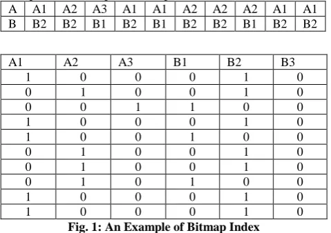
A bitmap for an attribute (column) of a table can be viewed as a m × n matrix, where m is the number of distinct values of the column and n is the number of tuples (rows) in the table. Each value in the column corresponds to a bitmap vector of length n, in which the kth position of the vector is 1 if this value appears in the kth row, and 0 otherwise. In this paper we use equality-encoded bitmaps. An example of bitmap index is shown in Figure 1. Table 1 shows an example relation with a set of attributes. Table2 shows the corresponding bitmap indices on attributes A and B of the table. For each distinct value of A and B, there is a corresponding bitmap vector. For instance, A1’s bitmap vector is 1001100011, because A1 occurs in the 1st, 4th, 5th, 9th and 10th rows in the table. An uncompressed bitmap can be much larger than the original data, thus compression is typically utilized

to reduce the storage size and improve performance. As reported above, with proper compression, bitmaps perform well for a column with cardinality up to 55% of the number of rows, that is, up to 55% of rows having distinct values in the column. We adopt Word-Aligned Hybrid (WAH) [24] to compress the bitmaps in our implementation.

A A1 A2 A3 A1 A1 A2 A2 A2 A1 A1 B B2 B2 B1 B2 B1 B2 B2 B1 B2 B2

A1 A2 A3 B1 B2 B3

1 0 0 0 1 0

0 1 0 0 1 0

0 0 1 1 0 0

1 0 0 0 1 0

1 0 0 1 0 0

0 1 0 0 1 0

0 1 0 0 1 0

0 1 0 1 0 0

1 0 0 0 1 0

1 0 0 0 1 0

Fig. 1: An Example of Bitmap Index

3.

PROPOSED WORK

This section proposes the research work that are used in query evaluation. In this we have used set operations like intersection and difference operations. In this we proposes the proposed algorithm to evaluate iceberg query using set operations.

SET OPERATIONS: A set is a common property among things and then gather up all the things that have common property. A set is a collection of distinct objects and that can not contain duplicate elements. You can combine multiple queries using the set operators UNION, INTERSECT and DIFFERENCE etc.

Set Intersection operation operates on two queries that return selected lists that share the exact position, number of columns, and data types. An intersection operation returns the rows from both queries that share the same values in all of the selected list columns.

The intersection operation for sets A and B gives the elements that are common to both sets A and B. For example set A has elements {2,4,5,7} and set B has elements {3,4,5,9}, then the result for the intersection of A and B is {4,5}. The difference of two sets A and B, written as A-B. A-B is the set of all elements of A that are not elements of B. The difference operation, along with union, intersection is an important and fundamental set theory operation.

For example set A has elements {1,2,3,4,5} and set B has elements {3,4,5,6,7,8}. Now the difference between A and B sets is

{1,2,3,4,5}-{3,4,5,6,7,8}={1,2}, same as the difference between B, A is B-A={3,4,5,6,7,8}-{1,2,3,4,5}={6,7,8}.

Proposed algorithm to evaluate iceberg query using set operations:

Iceberg (Attribute A, Attribute B, Threshold T)

Output: Iceberg results

1. generate Bitmaps(Attribute a, Attribute b)

2. For each vector a of Attribute A do

3. aset [], aset.countones, a.sp=find all one positions(a)

4. For each vector b of attribute B do

5. bset[], bset.countOnes, b.sp=find all positions(b)

6. while a ≠ null and b ≠ null do

7. countRes=0,

8.If(aset.countones>=threshold&& bset.countones>=threshold) then

9. do asset ∩ bset

10. If(countRes>Threshold) then

11.AddIcebergresult(a.value,b.value,countRes)into R

12. aset,bset=perform a-(a∩b)

13. acountones=getcount(asset)

14. bcountones=getcount(bset)

15. If(acountones>Threshold) then

16. Repeat from step 9 to 15 for a and b

17. endIf

18. Return R.

threshold, if it satisfies T, moved to next stage, otherwise removed directly from processing. In the next stage the common index positions are found by doing intersection between vectors of attributes A and B, if the result of intersection satisfies T, then that pair will be sent to the resultant iceberg query, and moved on to the next stage, otherwise removed from the processing. In the next stage the difference operation will be done to update the index positions of intersected vectors. If the updated vectors satisfy the T, then the above process will be repeated until completion of all bit map vectors.

Validation of index based algorithm on sample database:

We will illustrate our process using an iceberg query having two aggregate attributes with COUNT function as the running example. We will show how the algorithm can be adjusted to support other aggregation functions and arbitrary number of aggregate attributes. Suppose the iceberg query that we need to answer is as the one in Figure 2.

The data table and bitmap indices are as those in Figure 1. The naive way to process this iceberg query on two attributes A and B using bitmap indices is to find the bit positions of each attribute of A and B. For example, if A and B have I and J distinct values respectively, I*J set operations will be needed to produce the iceberg results. To reduce these I*J operations we will conduct preprocessing operation. From the below example we will illustrate our process.

SELECT A,B,COUNT(*) FROM R GROUP BY A,B HAVING COUNT(*) > 2

Fig. 2: An Iceberg Query with COUNT Function

Example 3.1: In table R, column A has 3 distinct values “A1, A2, A3”, and column B has 3 distinct values “B1,B2, B3”. The bitmap indices are those on the right of Figure 1. To process the iceberg query in Figure 2, the naive approach will conduct set intersection operations. In this we conduct intersection operations between 9 pairs: (A1,B1), (A1,B2), (A1,B3), (A2,B1), (A2,B2), (A2,B3), (A3,B1), (A3,B2) and (A3,B3). Before conducting the intersection operation we will conduct the pre processing step. In this we will check whether the bit positions of each attribute are greater than the specified threshold or not. After each preprocessing operation, if the numbers of bit positions are greater than the threshold T then we will conduct intersection operation between the pairs. If the number of bit positions of each attribute is less than the threshold we will discard the attribute. After each intersection operation if the number of 1 bit positions is larger than the threshold (2 in this example), it is added into the iceberg result set. After each intersection operation the attribute is updated by conducting the difference operation between the individual attribute and intersection pair. From the below example we will understand how the process will be done.

Example 3.2: Consider the bitmap vectors A1 =1001100011, B1 = 0010100100, A2=0100011100, B2=1101011011, A3=0010000000, B3=0000000000 of our running example in Figure 1. When we find bit positions and store them in a set we get A1={0,3,4,8,9} and B1={2,4,7}, A2={1,5,6,7}, B2={0,1,3,5,6,8,9}, A3={2}, B3={no bit positions}.

When we conduct preprocessing step we will check whether all bitmap vectors have number of bit positions greater than the threshold T(2).

A1’s number of bit positions=5>2

A2’s number of bit positions=4>2

A3’s number of bit positions=1<2

B1’s number of bit positions=3>2 B2’s number of bit positions=7>2

B3’s number of bit positions=0<2

From the above preprocessing step we will discard A3 and B3 and we will send remaining bitmap vectors for intersection operation. With this preprocessing step instead of doing 9 intersection operations we will conduct only 4 intersection operations. After preprocessing step we get the pairs for intersection are

(A1,B1),(A1,B2),(A2,B1),(A2,B2).

When we conduct intersection between A1,B1 we will get the below result.

A1={0,3,4,8,9}∩{2,4,7}={4}=1<2.

The number of bit positions of intersected bitmap vectors is less than the threshold, so we will discard the pair, without sending it to the resultant vector.

Now we will conduct the difference operation to A1,B1 vectors to update these bitmap vectors.

A1=A1-(A1∩B1)={0,3,4,8,9}-{4}={0,3,8,9}=4(number of bit positions)>2

B1=B1-(A1∩B1)={2,4,7}-{4}={2,7}=2(number of bit positions)<2

After each difference operation we adds an extra pruning step of monitoring the number of remaining 1s in both bitmap vectors involved. If the number of 1 bits of a modified vector becomes smaller than the iceberg threshold, this vector can be pruned. That is, no further intersection operation is necessary for this vector. With difference operation, the number of intersection operations can be reduced effectively, since the iceberg threshold is usually large. Now we will conduct intersection operation for the pairs (A1,B2),(A2,B2). By following the above process we will get the resultant pair as (A1,B2) and (A2,B2).

4.

IMPLEMENTATION

This section describes different models that were proposed in the previous section. In this section we propose the generation of bitmaps, finding bit positions, iceberg query evaluation using set operations like intersection and difference operations.

Step1: Generate bitmaps:

The first module generates bitmaps from input attributes; these generated output bitmaps are given as the input to the next module. The next module finds the index positions of all 1’s in the generated bitmap vectors.

Step 2: Findallindexpositions

This module finds all 1 bit positions of bitmap vector and stores the bit positions in to sets say aset{}, bset{}, and computes the count of index positions. This module checks whether the count satisfies the T or not.

Step 3: INTERSECTION operation

Step 4: DIFFERENCE OPERATION

After getting the results from the intersection operation the original bitmap vectors are updated by doing the difference operation. If the count of index positions are above T after updating the vectors will be future referenced, else pruned. The above modules are implemented using JAVA language for the purpose of experimentation.

5.

EXPERIMENTATION

This section describes the experiment to be carried out on the implementation described in the previous section under a specified iceberg threshold values that increase from 100 to 1000. The database tuples are 1.0 lakh. First the iceberg query is responsible to select the similar records with A and B attributes from the database table R which are having threshold value ranging between 100 and 1000. Then, the experiment is to be conducted by firing an iceberg query as stated in fig2. On the database table which consists of 1 lakh of tuples with two attributes A and B and COUNT as an aggregation function. The first function i.e., generatebitmaps accepts all these tuples as input. This function first produce bitmap vector from the given input attributes. Then the second function Findallindexpositions finds all the index positions of 1’s and store them in to sets. The COUNT function counts the bit positions of bitmap vectors. After counting the bitmap vectors positions the count will be checked with the threshold T(value greater than 100 to 1000). If T is satisfied then the intersection will be done by these satisfied pairs. If the result is satisfied by the T then the pair will be sent to the resultant iceberg. The actual vectors are updated after intersection operation by doing the difference operation. The experiment is repeated for different iceberg thresholds by keeping the same number of tuples in a database table and noted variations in execution times.

5.1

Results & Analysis

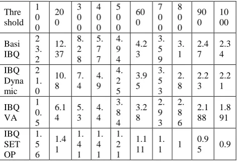
This section describes the results obtained in our experiment conducted in the previous section and are shown in below table.

The first column shows the different thresholds T. The second column shows the execution times recorded.

Thre shold 1 0 0 20 0 3 0 0 4 0 0 5 0 0 60 0 7 0 0 8 0 0 90 0 10 00 Basi IBQ 2 3. 2 12. 37 8. 2 8 5. 7 7 4. 9 4 4.2 3 3. 5 9 3. 1 2.4 7 2.3 4 IBQ Dyna mic 2 1. 0 10. 8 7. 4 4. 9 4. 2 5 3.9 5 3. 5 3 2. 8 2.2 3 2.2 1 IBQ VA 1 0. 5 6.1 4 5. 3 4. 4 3. 8 4 3.2 8 2. 9 3 2. 8 6 2.1 88 1.8 91 IBQ SET OP 1. 5 6 1.4 1 1. 4 1 1. 4 1 1. 2 1 1.1 11 1. 1 1

0.9 5 0.9

Fig4(a): Table showing execution time by varying thresholds The above result table in fig 4(a) consists of 5 rows and 11 columns. The first row showing the thresholds ranging from 100 to 1000. And second, third, fourth and fifth rows are different iceberg query evaluation algorithms such as Basic IBQ, IBQ Dynamic, IBQ PQ, and IBQSETOP respectively. All the respective column values are filled with execution time by changing the thresholds. The algorithm IBQ SETOP executing the iceberg query with minimum execution time for

all the thresholds compared with remaining algorithms which are existing in previous shown in the table.

Fig4(b): Graph showing comparison of execution time Vs Threshold

The above graph in fig4(b) is showing clear execution time of different algorithms existing in previous. The graph is having two axis titles horizontal and vertical on which threshold and execution time are shown respectively. The basic IBQ algorithm is evaluating iceberg queries at 100 threshold is with 23.0 milli seconds which is the highest execution time offered from all other algorithms. And the setop algorithm is the lowest execution time offered among all other algorithms. Similarly The graph is showing comparison of execution times versus thresholds ranging from 100 to 1000.

6.

CONCLUSION

This paper presents a new Framework which evaluates iceberg queries using bitmap indices and set operations. The main advantage of this method of evaluation is avoiding an execution of AND operations between unwanted bits of bitmaps. The setIntersection operation considers only index positions of one bits from each bitmap and perform the intersection operation between them to produce iceberg results. Thus inherently this method saves an execution time between all unwanted bits of bitmaps. The setDifference operation determines the future reference of the original bitmaps which are already involved in the intersection operation. These two simple set operations save maximum execution time when compared to existing algorithms that are shown by our extensive experimentation. The future research direction of this work may be reduction of number of set operations generated which optimizes the execution time of evaluation of iceberg queries.

7.

ACKNOWLEDGMENT

Our thanks to the management members and principal of Kakatiya Institute of Technology and Science-Warangal who have facilitated resources to read and compute in order to develop this article and our sincere thanks to Head of the Department Prof.P.Niranjan who encouraged us research and publish this paper.

8.

REFERENCES

[1] Bin He, Hui-I Hsiao, Ziyang Liu, Yu Huang and Yi Chen, “Efficient Iceberg Query Evaluation Using Compressed Bitmap Index”, IEEE Transactions On Knowledge and Data Engineering, vol 24, issue 9, sept 2011, pp.1570-1589

[2] D.E. Knuth, “The Art of Computer Programming : A Foundation for computer mathematics” Addison-Wesley

0 5 10 15 20 25

100 300 500 700 900

E x e . T i m e _Threshold

IBQ Evaluation:Threshold Vs Exe.Time

Basic IBQ

IBQ Dynamic

IBQVA

Professional, second edition, ISBN NO: 0-201-89684-2, January 10, 1973.

[3] G.Antoshenkov, “Byte-aligned Bitmap Compression”, Proceedings of the Conference on Data Compression, IEEE Computer Society, Washington, DC, USA, Mar28-30,1995, pp.476

[4] Hsiao H, Liu Z, Huang Y, Chen Y, “Efficient Iceberg Query Evaluation using Compressed Bitmap Index”, in Knowledge and Data Engineering, IEEE, Issue: 99, 2011, pp:1.

[5] Jinuk Bae,Sukho Lee, “Partitioning Algorithms for the Computation of Average Iceberg Queries”, Springer-Verlag, ISBN:3-540-67980-4, 2000, pp: 276 – 286.

[6] J.Baeand, S.Lee, “Partitioning Algorithms for the Computation of Average Iceberg Queries”, in DaWaK, 2000.

[7] K. P. Leela, P. M. Tolani, and J. R. Haritsa.”On Incorporating Iceberg Queries in Query Processors”, in DASFAA, 2004, pages 431–442.

[8] K.Stockinger, J.Cieslewicz, K.Wu, D.Rotem and A.Shoshani. “Using Bitmap Index for Joint Queries on Structured and Text Data”, Annals of Information Systems, 2009, pp: 1–23.

[9] K.Wu,E.J.Otoo and A.Shoshani. “Optimizing Bitmap Indices with Efficient Compression”, ACM Transactions on Database System, 31(1):1–38, 2006.

[10] K.Wu,EJ.Otoo,and A.Shoshani, “On the Performance of Bitmap Indices for High Cardinality Attributes”, VLDB, 2004, pp: 24–35.

[11] K.-Y.Whang, B.T.V.Zanden and H.M.Taylor.”A Linear-Time Probabilistic Counting Algorithm for Database Applications”. ACMTrans.Database Syst., 15(2):208– 229, 1990.

[12] M.Fang, N.Shivakumar, H.Garcia- Molina, R.Motwani and J.D.Ullman.”Computing Iceberg Queries Efficiently”. In VLDB, pages 299–310, 1998.

[13] M.Jrgens “Tree Based Indexes vs. Bitmap Indexes: A Performance Study” In DMDW, 1999.

[14] M.Stonebraker, D.J.Abadi, A.Batkin, X.Chen, M.Cherniack, M.Ferreira, E.Lau,A.Lin, S.Madden, E.J.O’Neil, P.E.O’Neil, A.Rasin, N.Tran and S.B.Zdonik.C-Store: “A Column-oriented DBMS”. In VLDB, pages 553–564, 2005.

[15] P.E.O’Neil.”Model204 Architecture and Performance”. In HPTS Pages 40–59, 1987.

[16] P.E.O’Neiland D.Quass. “Improved Query Performance with Variant Indexes”. In SIGMOD Conference, pages 38–49, 1997.

[17] P.E.O’Neil and G.Graefe. “Multi-Table Joins Through Bitmapped Join Indices”. SIGMOD Record, 24(3):8–11, 1995.

[18] R.Agarwal,T.Imilinski,andA.Swami.”MiningA ssociation Rules between Sets of Items in Large databases”. In SIGMOD Conference, pages 207-216, 1993.

[19] Spiegler I; Maayan R “Storage and retrieval considerations of binary databases”. Information processing and management: an international journal 21 (3): pages 233-54, 1985.

9.

AUTHOR’S PROFILE

Ch.Chaitanya Bharathi Currently persuing Master of Technology in Computer Science and engineering with specilization in Softwatre Engineering.Computer Science and Engineering Department, Kakatiya Institute of Technology & Science (KITS), Kakatiya University-Warangal.A.P.,India.

Vuppu Shankar obtained his Bachelor’s degree in Computer Technology from Nagpur University of India. Then he obtained his Master’s degree in Computer Science from JNTU Hyderabad, and he is also life member of ISTE,IEEE. He is currently an Associate Professor at the Faculty of Computer Science and Engineering, Kakatiya Institute of Technology & Science (KITS), Kakatiya University-Warangal. His specializations include Data mining and Data warehousing, Databases and networking. His current research interest in computation of an iceberg cubes and evaluation of iceberg queries efficiently.