Evaluation of Unlimited Storage: Towards Better Data Access Model for “Sensor Network"

11

Evaluation of

Unlimited

Storage: Towards Better Data

Access Model for “Sensor Network”

Sagar M Mane

Walchand Institute of Technology Solapur. India.

Solapur University, Solapur.

S.S.Apte

Walchand Institute of Technology Solapur. India.

Solapur University, Solapur.

ABSTRACT

In sensor network a large amount of data need to be collected for future information retrieval. The data centric storage has become an important issue in sensor network. Storage nodes are used in this paper to store and process the collected data. This paper considers the storage node placement problem aiming to place unlimited storage nodes in sensor network to minimize the total energy cost for collecting the raw data and replying queries at the storage nodes. In this paper a strong data access model for placing storage nodes in sensor network is presented. Here we consider an application in which sensor networks provide real time data services to user. The main aim of this paper is to reduce the cost for raw data transfer, query diffusion, query reply by defining the best location of storage nodes in sensor network.

Keywords

Wireless sensor network, data reduction rate, data storage, data reply, data query, query diffusion.

1. INTRODUCTION

One of the key challenges in wireless sensor network is the storage and querying of useful sensor data. The wireless sensor network is built of nodes, where each node is connected to one or more sensors. Sensor networks deployed for different computing applications. Storage is an essential factor of any data centric sensor network application. One of the main challenges in these applications is how to search and store the collected data. The collected data can either be stored in the network sensors, or transmitted back to the sink and stored there for future retrieval. This design is ideal since data are stored in a central place for permanent access. Placing unlimited storage nodes is related to the sensor network. Query is the most important part of sensor network since in aspect sensor network provides the information about environmental condition to the end user. The main aim of this paper is to minimize the total energy cost and data query by accurately deploying the storage nodes in sensor network.

2. RELATED WORK

There has been a lot of prior research work on data querying models in sensor network. In early models [1, 2, 3], query is

Spread to every sensor node by flooding messages. Sensors nodes send data back to the sink in the reverse direction of query messages. Those methods do not consider the storage concern in sensor networks.

Data-centric storage schemes [4, 5, 6] store data to different places in sensor networks according to different data types. In [5, 6], the authors propose a data-centric storage scheme for sensor networks, which inherits ideas from distributed hash table. The home site of a data is obtained by applying a hash function on the data type

LEACH [7] is a clustering based routing protocol, in which cluster heads can fuse the data collected from its neighbors to reduce communication cost to the sink. LEACH has a similar structure accomplished by us, having cluster heads aggregate and forward data to the sink. However, LEACH aims to reduce data transmission by aggregating data; it does not address storage problem in sensor networks

PRESTO [8] is a recent research works on storage architecture for wireless sensor networks. A proxy layer is introduced between sensor nodes and user terminals and proxy nodes can cache previous query responses. When a query arrives in a proxy node, it first checks if the cached data can satisfy the query before forwarding the query to other nodes. Compared with the storage nodes in this paper, Nodes in PRESTO have no resource constraints in term of computation, power, storage and communication. It is a more familiar storage architecture that does not take the characteristics of data generation or query into consideration.

3. Proposed Data Access Model

Volume 73– No.7, July 2013

  

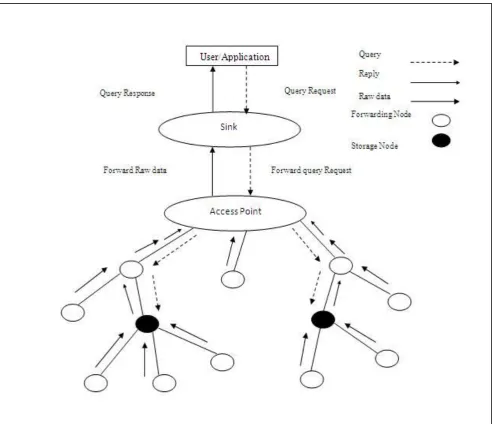
Figure 1: Data Access Model with Storage Nodes and Forwarding Nodes.



This requires each sensor to send its readings back to the Access point immediately every time it produces new data. Transferring all raw data could be very expensive and is not always required. Alternatively, allow sensors node to hold their raw data and to be aware of the different queries, then raw data can be managed to contain only the readings that users are interested in and the reduced reply size, instead of the whole raw data readings, can be send back to the sink. This design is illustrated in Fig. 1, where the black sensor nodes, called storage nodes, are allowed to hold raw data. The base station diffuses queries to the access point by broadcasting to the sensor network and then access point Broadcast the queries to storage sensors and these storage sensors reply to the queries by sending the processed data back to the storage node. Compared to the earlier solution, this approach reduces cost of the raw data transfer because some raw data transmissions are replaced by query reply.

On the other hand, this scheme incurs an extra query diffusion cost (as figured by the dashed arrows). In this paper, we are interested in vital designing a data access model to minimize energy cost associated with query diffusion, raw data transfers, and query replies.

Access Point: When the user fires the query on the sink, sink

forward the query Request to the access point. Access point broadcast the query to sensor nodes. When the query arrived at storage nodes they forward the raw data back to the access point and then access point obtain the result and forward the data to the sink..

First formally define two types of sensors (or nodes):

Storage nodes: These types of nodes have much larger

13 needed from the raw data they are holding and then return the

results back to the base station. The base station itself is considered as a storage node.

Forwarding nodes: These types of nodes are regular sensors

and they always forward the data received from other nodes or generated by themselves along a path towards the sink. The outgoing data are kept intact and the forwarding operation continues until the data reach a nearest storage node. The raw data forwarding operation is independent of queries and there is no data processing at forwarding nodes.

4. Placing Unlimited Number of

Storage nodes

Let i be any node in the communication tree and Ti be the subtree rooted at i. first use |Ti | to denote the number of Nodes in Ti . then define E(i) to be the energy cost incurred at i per time unit, which consist, the cost for raw data transfer i to its parent if i is a forwarding node, the cost for query diffusion if i has storage nodes as its descendants, and the cost for query reply if i is a storage node or has a storage descendant. To define E(i) mathematically we need to consider several possible cases.

Case I: i is a forwarding node and there are no storage nodes

in Ti . All raw data generated by the nodes in Ti have to be forwarded to the parent of i and there is no query diffusion cost. So E(i) = |Ti |Rd Sd .

Case II: i is a storage node and there are no other storage

nodes in Ti . The latest readings of all raw data generated by the nodes in Ti are processed at node i and the reduced reply size will be β|Ti |sd . Node i sends the reply to its parent when queries arrive. So E(i) = Rq β|Ti |Sd .

Case III. i is a storage node and there is at least one other

storage node in Ti . In addition to the cost for query reply as defined in Case II, i also incurs a cost for query diffusion that is implemented by broadcasting to its children. So E(i) = Rq β|Ti |Sd + Bi Rq Sq

Case IV. i is a forwarding node and there is at least one

Storage node in Ti . This is the case where all three types of cost (for query diffusion, raw data transfer, and query reply) are present. Among the |Ti |− 1 descendants of i, let d1 be the number of forwarding descendants without any storage nodes on their paths to i and d2 be the number of storage descendant’s or forwarding descendants with at least one storage node on their paths to i .

Obviously, d1 + d2 = |Ti |− 1. So

E(i) = (d1 + 1)Rd Sd + Bi Rq Sq + Rq βd2 Sd 1: make the root a storage node

2: if βRq ≥ Rd then

3: make all non-root nodes forwarding nodes and return 4: end if

5: for all leaves i do 6::make i a storage node 7: e*[i]=RqβSd 8: ef[i]=RdSd 9: end for

10: for all remaining nodes i do 11: make i a storage node

12: min1=Rqβ|Ti|Sd+BiRqSq+∑j€ci e*[j] 13: min2=Rqβ|Ti|Sd+∑j€ci ef[j]

14: e*[i]=min{min1,min2} 15: ef[i]=|Ti|RdSd+∑j€ci ef[j] 16: if min1≥min2 then

17: change each descendent of i that is a storage node to a forwarding node

19: end for

Algorithm 1: Placing unlimited storage nodes

Algorithm relies on following lemma.

Lemma 1.Given a node i and its sub tree Ti. If βRq≥Rd, then i must be a forwarding node to minimize e(i).if βRq≤Rd, then i must be a storage node to minimize e(i).

Proof: First compare the two trees based on their energy cost, which are equivalent in every aspect except that the first tree’s root is a forwarding node and the second tree’s root is a storage node. Let e1 and e2 be the two trees based on their energy cost. Comparing the two trees using the energy cost of individual nodes, one by one, observe that any two non- root nodes in the same position of the trees must have the similar energy cost. The only change is the energy cost of the roots. Let E1 and E2 be the energy cost of the roots in the two trees, respectively. Therefore, e1 − e2 = E1 − E2.

Here consider two cases. First, if both root have no storage descendants, then according to the four different case definition of energy cost (case I and II).

E1-E2 = |Ti| Rd Sd -Rqβ |Ti|Sd = Ti| Sd(Rd-βRq)

Second, if both roots have at least one storage descendant, then according to the four different case definition of energy cost (Cases III and IV).

E1-E2=((d1+1)RdSd+BiRqSq+Rqβd2Sd)– Rqβ|Ti|Sd+BiRqSq) = (d1+1)Sd(Rd-βRq).

From the above lemma, conclude that if βRq≥ Rd then every node (except for the root/sink, which is always a storage node) in the sensor network must be a forwarding node to minimize the energy cost.

The query diffusion cost can be eliminated if every subtrees of i has only forwarding nodes, i.e., E(i) = Rq β||Ti |Sd .(See Cases III and II in the four-case definition of E(i)) Thus, the minimum energy cost of the tree rooted at i should be derived from the better of these two scenarios

For a tree Ti rooted at i, let Ci be the set of children of i. Let e*(i) be the minimum energy cost of Ti . If Ci is empty, i.e., i is a leaf, then i must be a storage node to achieve its minimum energy cost. So e*(i) = Rq βSd . If Ci is not empty, then for any j € Ci , let ef (j) be the energy cost of Tj when all nodes in Tj are forwarding nodes. So

e∗ (i) = min {Rq β |Ti |Sd + Bi Rq Sq +∑j€ci e∗(j) ,

Rq β|Ti| Sd +∑j€ci ef (j) }.

From the design of the algorithm, we also observe that every node starts as a storage node and that once it is changed to a forwarding node, it will never be changed back. Therefore, all its descendants are replaced to forwarding nodes as well. it is impossible for a forwarding node to have a storage node descendant. Likewise, it is impossible for a storage node to have a forwarding node ancestor.

Volume 73– No.7, July 2013

Figure 2: Placing unlimited number of storage nodes flow chart.

No

No

No

No

Start

Make root as

storage node

If

βRq≥Rd

Make all non root

nodes forwarding

nodes

Input Rd,Rq,Sd,Sq,β

i=1

Make i a

storage

node 1

All leaves i=1

Storage node 1

i=i+1

Storage node 1

1

ef[i]= RdSd e*[i]= RqβSd

Exit

Storage node 2

min 2= Rqβ|Ti|Sd+∑j€ci ef[j]

min 1= Rqβ|T i|Sd + BiRqSq +∑j€ci e*[j]

Exit

ef[i ]=|Ti|RdSd+∑j€ci

ef[j]

e*[i]=min{min1,min2}

Change each

descendent of i

that is storage

to forwarding

node

All remaining

nodes i

Storage node 2

i=i+1

Stop

Make i a

storage

node 2

15 In this paper we consider the problem of storage node

placement in sensor network where the number of storage node is unlimited. Table 1 lists the notations, which we have used in this algorithm.

Table 1: Notations

5. RESULTED GRAPHS

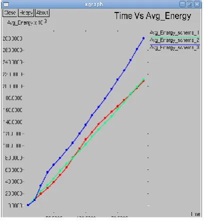
In our simulation settings, we consider a network of sensor deployed on a disk of radius 5 with the sink placed at the center. One hundred and one sensor nodes(n=101)are deployed to the field randomly. After all nodes are deployed in a routing tree rooted at the sink is constructed by broadcasting a message from the sink to all the nodes in the network. Therefore, for a certain set of parameters, we conduct several independent trials and the total average energy cost is used in the following analysis and comparison. We set the following parameters in our simulations: Rd=0.5,Rq=0.4,Sd=512,Sq=512.we evaluate the energy cost by varying the data reduction rate β.To simplify the description, we set Rd,Rq,Sd,Sq and only compute data reduction rate β to examine characteristics of data and queries.

Fig.3 indicates the comparison of unlimited storage nodes with Storage nodes vs. Total energy cost and other schemes. The xgraph values are taken from observations made from Algorithm 1.Where the graph of the average energy cost of unlimited storage nodes is indicated as red color.

Figure 4: Comparison of Unlimited storage nodes Storage nodes vs. Total Energy cost with other Schemes

Fig.4 indicates the comparison of unlimited storage nodes with the storage node vs. total energy cost and other schemes. The xgraph values are taken from observations made from Algorithm 1.Where the xgraph of unlimited storage nodes is indicated as red color.

Figure 3: Comparison of Unlimited storage nodes Time vs. Avg Energy cost with other schemes

Figure 5: Comparison of Unlimited storage nodes Time vs. Jitter with other schemes

Rd:-Data generation rate

Sd : Size of each data

ci : the number of node i’s children Rq: User query rate

Sq : size of each query message n: total number of sensors

e(i):Energy cost of all the nodes in Ti.

E(i): energy cost of node i

β: Data reduction rate

Volume 73– No.7, July 2013

16

Fig.5 indicates the comparison of unlimited storage nodes with Time vs. Jitter and other schemes. The xgraph values are taken from observations made from Algorithm 1.Where the graph of unlimited storage nodes is indicated as red color.

6. CONCLUSION AND FUTURE WORK

This paper considers the storage node placement problem in a sensor network. This paper introduces unlimited number of storage nodes in sensor network release the cost of sending all the raw data to a central place. In this paper, first examine how to place unlimited number of storage nodes to save energy for data collection and data query. This new model is much more simplified and implementable. We have tested it on different data sets available on internet using network simulator software. Our Future work includes Evaluation of limited number of storage nodes in sensor network to optimize query reply in a sensor network and to solve the storage node placement problem in terms of other performance metrics.

7. REFERENCES

[1] C. Intanagonwiwat, R. Govindan, and D. Estrin. rected diffusion: a scalable and robust Communication paradigm for sensor networks. In Proceedings of the 6th annual international conference on Mobile computing and networking, pages 56–67, New York, NY, USA, 2000. ACM Press

[2] C. Intanagonwiwat, R. Govindan, D. Estrin, J. Heidemann, and F. Silva. Directed diffusion for wireless sensor networking. IEEE/ACM Trans. Netw., 11(1):2– 16, 2003.

[3] S. Madden, M. J. Franklin, J. M. Hellerstein,and W.Hong TAG: a tiny aggregation service for ad-hoc sensor networks.SIGOPS Opererating System Review, 36(SI):131146,2002

[4] J. Newsome and D. Song. GEM: graph embedding for routing and data-centric storage in sensor networks without geographic information. In Proceedings of the 1st international conference on Embedded networked sensor systems, pages 76–88, New York, NY, USA, 2003.ACM Press.

[5] S. Ratnasamy, B. Karp, S. Shenker, D. Estrin, R. Govindan, L. Yin, and F. Yu. Data-centric storage in sensornets with GHT, a geographic hash table. Mobile Networks and Applications, 8(4):427–442, 2003.

[6] S. Shenker, S. Ratnasamy, B. Karp, R. Govindan, and D. Estrin. Data-centric storage in sensornets. SIGCOMM Computer Communication Review, 33(1):137–142, 2003.

[7] W. Heinzelman, A. Chandrakasan, and H. Balakrishnan.Energy-efficient Communication Protocols for Wireless Microsensor Networks. In International Conference on System Sciences, Maui, HI, January 2000.

[8] P. Desnoyers, D. Ganesan, H. Li, M. Li, and P. Shenoy. PRESTO: A predictive storage architecture for sensor networks. In Tenth Workshop on Hot Topics in Operating System, 2005.

[9] P. Gupta and P. R. Kumar. The capacity of wireless networks IEEE Transactions on Information Theory, IT- 46(2):388–404March 2000.

[10] D. Ganesan, D. Estrin, and J. Heidemann. Dimensions: why do we need a new data handling architecture for sensor networks?SIGCOMM Comput. Commun. Rev., 33(1):143– 148, 2003.

[11] E. J. Duarte-Melo and M. Liu. Data-gathering wireless Sensor networks: organization and capacity . Computer Networks (COMNET), 43(4):519–537, Nov. 2003