Diagnosis of Breast Cancer using Decision Tree Models
and SVM
Alaa M. Elsayad
Computers and Systems Dept,Electronics Research Institute, Cairo, Egypt.
Electrical Engineering Dept, Engineering College,
Salman University,
Saudi Arabia.
H.A. Elsalamony
Mathematics Dept., Faculty ofScience, Helwan University, Cairo, Egypt.
Computer Science & Information Dept., Arts & Science College, Salman University, Saudi Arabia.
ABSTRACT
Breast cancer represents the second important cause of cancer deaths in women today and it is the most common type of cancer in women. Disease diagnosis is one of the applications where data mining tools are proving successful results. Data mining with decision trees is popular and effective data mining classification approach. Decision trees have the ability to generate understandable classification rules, which are very efficient tool for transfer knowledge to physicians and medical specialists. In fundamental truth, they provide trails to find rules that could be evaluated for separating the input samples into one of several groups without having to state the functional relationship directly. The objective of this paper is to examine the performance of recent invented decision tree modeling algorithms and compared with one that achieved by radial basis function kernel support vector machine (RBF-SVM) on the diagnosis of breast cancer using cytological proven tumor dataset. Four models have been evaluated in decision tree: Chi-squared Automatic Interaction Detection (CHAID), Classification and Regression tree (C&R), Quick Unbiased Efficient Statistical Tree (QUEST), and Ross Quinlan new decision tree model C5.0. The objective is to classify a tumor as either benign or malignant based on cell descriptions compound by microscopic examination using decision tree models. The proposed algorithm imputes the missing values with C&R tree. Then, the performances of the five models are measured by three statistical measures; classification accuracy, sensitivity, and specificity.
General Terms
Breast cancer, Data miningKeywords
Breast cancer; classification, decision tree algorithms; SVM; missing data imputation
1.
INTRODUCTION
Breast cancer is the most common cancer among females. It is the second most important cause of death among women, as it comes directly after lung cancer [5]. The disease is characterized by malignant tumors when cells in the breast tissue divide and grow without normal controls on cell death and cell division [14]. In fact, it is the most common form of cancer in females; that is affecting approximately 10% of all them at some period of their life. The breast cancer attacks the Arab countries in the last ten years compared with other countries. The disease targets women in Arab countries of age of 30, while infecting women above 45 years in European countries [3]. Although scientists do not know the exact causes of most types of breast cancer, they know some of the
risk factors that increase the probability of woman infection, such attributes are: age, genetic risk and family history.
Medical scientists consider that mammography screening as the most dependable method of early detection of breast cancer. Nevertheless, the digital mammogram images are sometimes difficult to be read due to their low contrast and differences in the types of tissues [5]. In such cases, fine needle aspiration cytology is adopted. The tissue has to be removed for examination using breast biopsy techniques. A false positive detection may cause an unnecessary biopsy. Statistics show that only 20-30 percentages of breast biopsy cases proved cancerous [3]. A false negative detection, an actual tumor remains hidden that could lead to higher costs or even to the cost of a human life. However, the existing tumors are of different types, different shapes and some of them have the individuality of the normal tissue. So, it is necessary to develop better identification methods to recognize breast cancer.
Data mining methods can help to reduce the number of false positives and false negative decisions [16, 18, 19, 24]. The objective is to assign patients to either a ‘benign’ group that does not have breast cancer or a ‘malignant’ group that has strong evidence of having breast cancer based on cytological proven tumor data. Decision tree approaches are the most widely used data mining methods for several reasons. It has the ability to generate understandable rules, and to handle both continuous and categorical variables [8]. This paper investigates the effectiveness of four efficient decision tree models (C&R, CHAID, QUEST, and C5.0) on the diagnosis of the Wisconsin Breast Cancer dataset. The results are compared to those obtained using radial basis function kernel support vector machine (RBF-SVM). SVM has been chosen as it is considered a good candidate because of its high generalization performance [10].
maintains all other values that are heterogeneous (dissimilar or impure). C&R tree algorithm was popularized by Breiman, Friedman, Olshen, and Stone in 1984 [2] and by Ripley in 1996 [25]. The algorithm uses have the ability to use Gini or towing impurity measures for symbolic (categorical) target. The third decision tree mode QUEST is named from Quick, Unbiased, and Efficient Statistical Tree. It can be used with linear combination splits. QUEST is a binary-split decision tree algorithm for classification and data mining developed by Wei-Yin Loh and Yu-Shan Shih in 1997 in [21]. The fourth model is C5.0 decision tree, which is a recently invented modeling algorithm and it is an improved version of C4.5 and ID3 algorithms. C5.0 is a commercial product designed by Rule Quest Research Ltd Pty to analyze huge datasets and is implemented in SPSS Clementine workbench data mining software [12, 15].
The remainder of the paper is organized as follows: Section 2 describes the cytological attributes included in the dataset. Section 3 presents the four classifications DT models. RBF-SVM will show in Section 4. Section 5 presents the statistical measures used to evaluate the classification performance for all models and their experimental results. Finally, the conclusion will be discussed.
2.
DATA SET DISCRIPTION
This paper employed the Wisconsin Breast Cancer dataset from the University of California at Irvine (UCI) Machine Learning Repository has been used to evaluate the performances of four decision tree classification models. The breast cancer dataset used here was collected by Dr. William H. Wolberg (1989–1991) at the University of Wisconsin– Madison Hospitals [13]. Actually, the diagnosis of Wisconsin breast cancer has been attracting many researchers. Searching the ScienceDirect electronic library in November 2012, for "Breast and Cancer and Wisconsin and Diagnosis" keywords, resulted in 3,926 articles.
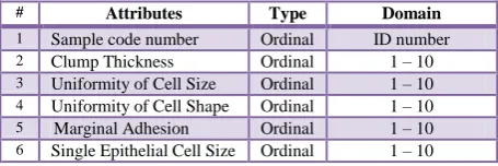
[image:2.595.315.543.71.134.2]The Wisconsin dataset contains 699 samples with 683 complete data and 16 samples with missing attributes. The samples were virtually assessed nuclear features of fine needle aspirates taken from patients' breasts. Each sample record has nine cytological attributes; they measure the external appearance and internal chromosome changes in nine different scales. The nine attributes are graded on an interval scale from a normal state of 1–10, with 10 being the most abnormal state [13]. The class attribute was represented as 2 for benign and 4 for malignant cases. All attribute values have the same range and there is no need for normalization as in Table 1.
Table 1. Wisconsin breast cancer dataset attributes
# Attributes Type Domain
1 Sample code number Ordinal ID number
2 Clump Thickness Ordinal 1 – 10
3 Uniformity of Cell Size Ordinal 1 – 10
4 Uniformity of Cell Shape Ordinal 1 – 10
5 Marginal Adhesion Ordinal 1 – 10
6 Single Epithelial Cell Size Ordinal 1 – 10
7 Bare Nuclei Ordinal 1 – 10
8 Bland Chromatin Ordinal 1 – 10
9 Normal Nucleoli Ordinal 1 – 10
10 Mitoses Ordinal 1 – 10
11 Class Flag 2 = benign,
4 = malignant
Table 2 introduces the value distributions of the nine microscopic attributes between benign and malignant cases. These percentages between benign and malignant classes ensure that lower values tend to be benign and higher values be likely malignant. The Clump thickness benign cells tend to be grouped in mono-layers, while malignant cells are often grouped in multi-player. From the values in this attribute, we noticed that about 86.123% of patients, which they have values ranged (1:5) are benign. While in the Uniformity of cell size/shape the cancer cells tend to vary in size and shape. On the Uniformity of Cell Size, about 92.704% from the patients’ those having values ranged (1:3) are benign, in addition the patients that they have values more than 3 at this attribute are malignant. Also, Uniformity of Cell Shape attribute's value (1:3) with ratio 92.275% lead to the patients are benign. In the case of Marginal adhesion, the normal cells tend to stick together, where cancer cells tend to lose this ability. So the loss of adhesion is a sign of malignancy. By applying this to the data in this attribute we can notice that, about 86.409% of values in the interval (1:3) are benign. Regarding the Single Epithelial Cell Size the size is related to the uniformity. The Epithelial cells that are significantly enlarged may be a malignant cell.
Correspondingly, if the attribute values fall in interval (1:3) by ratio 87.554% of patients will be benign, and it will be represented as a malignant patient otherwise. The Bare Nuclei is a term used for nuclei that is not surrounded by cytoplasm (the rest of the cell). Those are typically seen in benign tumors. This attribute has 16 missing values, then after imputing these missing data by C&R algorithm (in the experimental result section) we can note that most benign patients take the values between (1:5) by percentage less than the others in the previous 61.23%. For Bland Chromatin, this attribute describes a uniform "texture" of the nucleus seen in benign cells. In cancer cells the chromatin tends to be coarser.
[image:2.595.53.281.602.678.2]Table 2. Wisconsin breast cancer dataset attributes’ value percentages
V
a
lu
es
A
tt
ri
b
u
te
Clump Thickness
Uniformity of Cell Size
Uniformity of Cell Shape
Marginal Adhesion
Single Epithelial Cell Size
Bare Nuclei Bland Chromatin
Normal
Nucleoli Mitoses
M B M B M B M B M B M B M B M B M B
1
M
ali
gn
a
n
t=241,
B
en
ign
=
458
2% 98% 1% 99% 0.6% 99.4 8% 92% 2% 98% 30% 70% 1% 99% 9% 91% 23% 77%
2 8% 92% 18% 82% 12% 88% 36% 64% 6% 94% 35% 65% 4% 96% 17% 83% 77% 23%
3 11% 89% 48% 52% 41% 59% 47% 53% 60% 40% 45% 55% 22% 78% 73% 27% 94% 6%
4 15% 85% 77% 23% 70% 30% 85% 15% 85% 15% 30% 70% 80% 20% 94% 6% 100% 0%
5 35% 65% 100% 0% 91% 9% 83% 17% 87% 13% 50% 50% 88% 12% 89% 11% 83% 17%
6 53% 47% 93% 7% 90% 10% 82% 18% 95% 5% 75% 25% 90% 10% 82% 18% 100% 0%
7 96% 4% 95% 5% 93% 7% 100% 0% 75% 25% 75% 25% 90.% 10% 87% 13% 89% 11%
8 91% 9% 97% 3% 96% 4% 100% 0% 90% 10% 62% 38% 100% 0% 83% 17% 88% 12%
9 100% 0% 83% 17% 100% 0% 80% 20% 100% 0% 67% 33% 100% 0% 94% 6% 50% 50%
10 100% 0% 100% 0% 100% 0% 98% 2% 97% 3% 33% 67% 100% 0% 100% 0% 100% 0%
3.
DECISION TREE MODEL
ALGORITHMS
Fig.1. Illustrated example of binary decision tree
Decision tree (DT) provides powerful techniques for classification and prediction. There are several algorithms to build DT model [12, 23]. As the name implies, this model recursively separates data samples into branches to construct a tree structure for the purpose of improving the prediction accuracy. Each tree node is either a leaf node or decision node. All decision nodes have splits, testing the values of some functions of data attributes. Each branch of the decision node corresponds to a different outcome of the test. Each leaf node has a class label attached to it as shown in Figure 1. General algorithm to build a DT is as follows:
Start with the entire training subset and a vacant tree. If all training samples at the current node n are of the
same class label c, then the node becomes a leaf node with label c.
Or else, select the splitting attributes that is the most important in separating the training samples into different classes. This attribute becomes a decision node. A branch is created for each distinct value of s, and the
samples are partitioned accordingly.
The process is iterated recursively until a certain value of specified stopping criterion is achieved.
Different DT models use different algorithms to find attribute-threshold pairs that maximize the purity of the resulting two or more classes of data samples [8]. This paper evaluated four efficient DT learning models; Chi-squared automatic interaction detector (CHAID), classification and regression tree (C&R), quick, unbiased, efficient statistical tree (QUEST), and Commercial version 5.0 (C5.0).
3.1
Chi-squared Automatic Interaction
Detector (CHAID)
CHAID tree model relies on the Chi-square x2 Test to determine the best split at each step. The algorithm only accepts nominal or ordinal categorical predictive attributes [17]. When predictors are continuous, they are transformed into ordinal ones. Ordinal attribute is ordered set with intrinsic ranking. The CHAID DT modeling algorithm is as follows [1]:
Binning the continuous attribute (if exists) to create a set of categories, where each category is a sub-range along the entire range of the attribute. This binning operation permits the model to accept both categorical and continuous inputs, although it internally works only with categorical ones.
Analyzing the categories of each attribute to determine which ones can be merged safely to reduce the number of categories.
Computing the adjusted p-value for the merged categories by applying Bonferroni adjustments (it is a method used to counteract the problem of multiple comparisons).
Searching for the split point with the smallest adjusted p-value (probability p-value, which can be related to significance) to find the best split.
In step 2, the algorithm merges values that are judged to be statistically homogeneous (similar) with respect to the target attribute and maintains all other values that are heterogeneous (dissimilar). If the p-value is greater than specified parameter αmerg then the algorithm merges the pair of categories into a single one. The value of αmerg must be greater than 0 and less than or equal to 1. To prevent any merging of categories, specify a value of 1. In step 4, each predictive attribute is evaluated for its association with the target attribute, based on the adjusted p-value of the statistical test of association. Decision Node
(Root Node)
Leaf Node Internal Node
Internal Node
Leaf Node Leaf Node
Leaf Node
[image:3.595.80.212.311.461.2]The predictive attribute with the strongest association, indicated by the smallest adjusted p-value, is compared to a pre-specified split threshold αsplit. If the adjusted p-value is less than or equal to αsplit that attribute is selected as the split attribute of the current node. After the split is applied to the current node, the child nodes are examined to see if they warrant splitting by applying the merge/split process to each in turn. Processing proceeds recursively until one or more stopping rules are triggered for every non split node, and no further splits can be made. In this study, the target attribute is of categorical type (malignant or benign). The Likelihood ratio has been used to compute the chi-square statistic. The algorithm forms a contingency (count) table using the classes of the target attribute y as columns and the categories of the predictive attribute x as rows. The expected cell frequencies under the null hypothesis of independence are estimated. The observed cell frequencies and the expected cell ones are used to calculate the chi-squared statistic and the p-value.
(1)
where
Is the observed cell frequency andm
ijis the expected cell frequency in cells)
,
(
x
n
i
y
n
j
, and the p- value is computed as:(2)
The CHAID tree model is fast, builds “wider” decision trees as it is not constrained to make binary splits; making it very popular in different application. The model can be conveniently summarized in a simple two-way contingency table, with multiple categories for each variable. However, this algorithm requires larger quantities of data to get dependable results.
3.2
The Classification and Regression
(C&R) Tree
The C&R tree algorithm generates a regression model or a classification model depending on whether the target attribute is continuous or categorical.
Regression Models, if the target attribute is continuous, a regression model is generated. When using a regression tree to predict the value of the target attribute, the mean value of the target attribute of the rows falling in a terminal (leaf) node of the tree is the predicted value.
Classification Models, if the target attributed is categorical, then a classification model is generated. To predict the value (category) of the target attribute using a classification tree, use the values of the predictor attributes to move through the tree until you reach a terminal (leaf) node, then predict the category shown for that node.
C&R tree models recursively partition the data to find increasingly homogeneous subsets based on independent attribute splitting criteria using variance minimizing algorithms. The dependant data is partitioned into a series of descending left and right child nodes derived from parent
nodes [2]. C&R tree has the ability to use different measures of purity. We choose the Gini index, which is based on probabilities of category membership in the branch. The goal of tree building is to create subgroups with similar output values; in other words, to minimize the impurity within each node. If the best split for a branch reduces the impurity by less than the specified amount, the split will not be made. Gini Impurity Measure:
The Gini index at node t, g (t), is defined as:
(3)
where i and j are categories of the target attribute.
(4)
(5)
(6)
where
is the prior probability value for category
is the number of samples in category of node
and Is the number of samples by category in the root node. In addition, the Gini index is used to find the improvement for a split during tree growth, only those records in node and the root node with valid values for the split-predictor are used to compute
and , respectively. The equation for the Gini index can also be written as:
(7)
Thus, when the cases in a node are evenly distributed across
the categories, the Gini index takes its maximum value of
, where is the number of categories for the target attribute. When all cases in the node belong to the same category, the Gini index equals 0. Moreover, the Gini criterion function to split at node is defined as:
(8)
where is the proportion of records in sent to the left child node, and is the proportion sent to the right child node. The proportions and are defined as:
, and
(9)
The split is chosen to maximize the value of .
3.3
Quick, unbiased, efficient statistical
tree (QUEST)
QUEST uses an unbiased attribute selection technique. QUEST uses imputation instead of surrogate splits to
deal with missing values.
QUEST can easily handle categorical predictor attributes with many categories.
The QUEST modeling process consists of the selection of a split predictor, selection of a split point for the selected predictor, and stopping and only univariate splits are considered. In this application all the independent attributes are categorical type and the QUEST selection of split predictor uses the following algorithm [20].
For each categorical predictor , perform a Pearson’s chi- square test of dependent attribute and calculate the p-value according to the statistics. Find the predictor with the smallest p-value and
denote it .
If this smallest p-value is less than , where is a user specified level of significance and M is the total number of predictor attributes, predictor is selected as the split predictor for the node. If not, go to next step.
Find the predictor with the smallest p-value and denote it as .
is selected as the split predictor for the node. Otherwise, this node is not split.
3.4
Commercial version 5.0 (C5.0)
C5.0 is an improved version of C4.5 and ID3 algorithms [15]. It is a commercial product designed by Rule Quest Research Ltd Pty to analyze huge datasets and is implemented in SPSS Clementine workbench data mining software [3]. C5.0 uses common splitting algorithms include Entropy based information gain. The gain ratio is a robust and consistently gives a better choice of tests than the gain criterion (ID3) for large datasets. The model works by splitting the sample based on the attribute that provides the maximum information gain. Each subsample defined by the first split is then split again, usually based on a different attribute, and the process repeats until the subsamples cannot be split any further. Finally, the low-level splits are reexamined, and those that do not contribute significantly to the value of the model are removed or pruned.
C5.0 model is quite robust in the presence of problems such as missing data and large numbers of input fields. It usually does not require long training times to estimate. In addition, C5.0 models tend to be easier to understand than some other model types since the rules derived from the model have a very straightforward interpretation. C5.0 also offers the powerful boosting method to increase accuracy of classification [26].
C5.0 uses information gain as a measure of purity, which is based on the notion of entropy. If the training subset consists of n samples (x1, y1),…, (xn, yn), xi ϵ Rp is the independent
attributes of the sample i and yi is a predefined class
Y={c1,c2,…,ck}. Then, the entropy, entropy(X), of the set X
relative to this n-wise classification is defined as:
(10)
where pi is the ratio of X fitting in class ci.
The gain (X, A) is simply expected reduction in entropy caused by partitioning the set of samples, X, based on an attribute A:
(11)
where values (A) is the set of all possible values of attribute A, and Xv is the subset of X for which attribute A has the attribute
value v, i.e., Xv = {x X | A(x) = v}. Boosting, winnowing and
pruning are three methods used in the C5.0 tree construction; they propose to build the tree with the right size [16, 17]. They increase the generalization and reduce the over fitting of the DT model.
4.
SUPPORT VECTOR MACHINE(SVM)
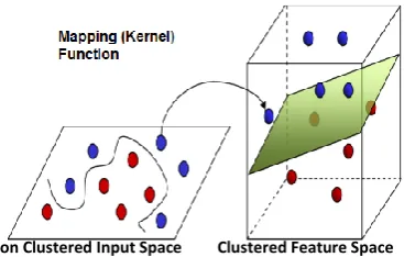
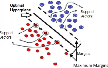
[image:5.595.321.505.510.627.2]The SVM model is a supervised machine learning technique, which is based on the statistical learning theory. It was firstly proposed by Cortes and Vapnik from his original work on structural risk minimization in [4] and modified by Vapnik in [28]. The algorithm of SVM is able to create a complex decision boundary between two classes with good classification ability. Figures 2 and 3 give the basic principles of SVM. When the data are not linearly separable, the algorithm works by mapping the input space to higher dimensional feature space, through some nonlinear mapping chosen a priori shown in Figure 2, and constructs a hyperplane, which splits class members from non-members as in Figure 3. SVM introduces the concept of ‘margin’ on either side of a hyperplane that separates the two classes. Maximizing the margins and thus creating the largest possible distance between the separating hyperplane and the samples on either side, is proven to reduce an upper bound on the expected generalization error. SVM may be considered a linear classifier in the feature space. On the other side it becomes a nonlinear classifier as a result of the nonlinear mapping from the input space to the feature one [9, 7].
Fig 2. Mapping the input space without clustering to a higher dimensional feature space.
Fig 3. Optimal hyperplane separating the two classes and support vectors
In the case of linearly separable classes, SVM divides these classes by finding the optimal (with maximum margin) separating hyperplane. Optimal hyperplane can be found by solving a convex quadratic programming (QP) problem [10]. Once the optimal separating hyperplane is found, data samples that lie on its margin are known as support vectors. The solution to this optimization problem is a global one.
For linearly decision space, suppose the training subset consists of n samples (x1, y1),…,(xn, yn), x Rp and y {+1,-1}
i.e. the data contain only two classes. The separating hyperplane can be written as:
b
wx
x
D
(
i)
i
w (12)where the vector w and constant b are learned from a training subset of linearly separable samples. The solution of SVM is equivalent to solve a linear constrained quadratic programming problem as an Equation (13) for both targets y equal (-1) and (1):
,
1
wx
b
y
i i i=1,…,n. (13)As mentioned before, samples that provide the above formula in case of equality are referred as support vectors. SVM classifies any new sample using these support vectors. On the other hand, the margins of the hyperplane follow the subsequent inequality:
, ) (
w x D
yi i i=1,…,n (14)
The norm of the w has to be minimized in order to maximize the margin
. In order to lessen the number of solutions to the norm of w, the following equation is assumed:1
w
(15) Then the algorithm tries to minimize the value of 22 /
1 w
subject to the conditions in Equation (13). In the case of non-separable samples, slack parameters ξ are added into Equation (13) as follows:
)
1
(
wx
b
y
i i ,
0
,
i
(16)And the value that needs to be minimized becomes:
n
i
i w
C 1
2
. 2 / 1
(17)where C is the regularization parameter. A regularization parameter C (may be called cost parameter) is a set to determine the level of tolerance the model has, with larger C
values allowing larger deviations from the optimal solution. This parameter is optimized to balance the classification error with the complexity of the model. There is a family of kernel functions that may be used to map input space into feature space. They range from simple linear and polynomial mappings of sigmoid and radial basis functions (RBFs). Once a hyperplane has been created, the kernel function is used to map new samples into the feature space for classification. This mapping technique makes SVM dimensionally independent, whereas other machine learning techniques are not. This paper uses the RBF kernel to map the input space into the higher dimensional feature space. RBF kernels can be controlled by adjusting the width of the basis functions
, so only one parameter that needs to be optimized [6].), / exp(
) ,
(x x xx 2 2
K (18)
where
is a specified positive real number, which determines the width of the RBF kernel. So, this RBF-SVM classification model has two parameters which need to be optimized; the width of the basis function
and the regularization parameter C [22]. The next section will show the experimental results for the proposed stream.5.
THE EXPERIMENTAL RESULTS
The performance of each classification model is evaluated using three statistical measures; classification accuracy, sensitivity and specificity. These measures are defined using true positive (TP), true negative (TN), false positive (FP) and false negative (FN). A true positive decision occurs when the positive prediction of the classifier coincided with a positive prediction of the physician. A true negative decision occurs when both the classifier and the physician suggest the absence of a positive prediction. False positive occurs when the system labels benign case as a malignant one. Finally, falsification negative occurs when the system labels a positive case as negative (benign). Classification accuracy is defined as the ratio of the number of correctly classified cases and is equal to the sum of TP and TN divided by the total number of cases N [11].
(19)
Sensitivity refers to the rate of correctly classified positive and is equal to TP divided by the sum of TP and FN. Sensitivity may be referred as a True Positive Rate
(20)
Specificity refers to the rate of correctly classified negative and is equal to the ratio of TN to the sum of TN and FP [11].
(21)
Clementine uses client/server architecture to distribute requests for resource-intensive operations with powerful server software, resulting in faster performance on larger
[image:7.595.63.543.90.224.2]datasets [12]. The software offers many modeling techniques, such as prediction, classification, segmentation, and association detection algorithms.
Fig.4 Data mining stream for the prediction of the severity of breast cancer using C&R, CHAID, QUEST, C5.0, and SVM respectively.
The breast Cancer dataset node is connected directly to an EXCEL sheet file that contains the source data. The data set was explored as an ordinal data type, and missed values. All of these missing values were falling in the attribute of Bari Nuclei. They are 16 missing values were appeared as null values. These null (missing) values will predict by using C&R algorithm
The type node specifies the field metadata and properties that are important for modeling and other work in Clementine. These properties include specifying usage type, setting options for handling missing values, as well as setting the role of an attribute for modeling purposes; input or output. As previously stated, the first 9 attributes in table 1 are defined as input (predictive) attributes and the Class attribute is defined as a target.
The Missing Values Super Node is used to represent the imputation and prediction of these 16 missing values using C&R algorithm. The missing data are predicted by putting the Bari Nuclei attribute, which has all the missing values, as a target with respect to other attributes.
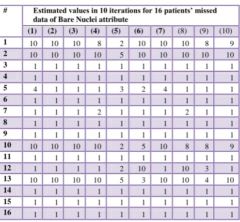
Table 3 illustrates the estimation of missing values, which appear in the dataset. In this table, 10 iterations have carried out to get the best one based on matching the other attribute context values. Moreover, Table 4 introduces a comparison of all 10 iterations, showed in table 3, of predicted matching values in Bare Nuclei attribute. These matching values lead to percentage ratios of matching according to the Class attribute (the decision column in the original dataset). In this table, the predicted values are stable with respect to CHAID model by ratio 81.25% for 13 matched values out of 16. In fact, the strong matching of these 10 iterations is coinciding of 14 predicted values by 87.5%, these values are appearing in only two models of the decision tree, C&R and C5.0, and SVM. According to information on this table, the importance of C&R and C5.0 is appeared on the predicted missing values with respect to CHAID and QUEST models. In the same context, the iterations are hesitating in values between two percentage ratios 75% and 87.5% in matching.
Although some of the predictive missing value has not led to the same Class attribute’s value in the dataset, it is in the same context of the attribute’s values for the same patient. For example, one patient appeared (from these three not matched), who its class value in the original data leads to benign, while in our prediction of missing values in the final result he is
[image:7.595.305.551.353.589.2]malignant. In addition, the characteristics of all attribute values for this patient are matching among the predictive value, which it is leading to the opposite (malignant) with the Class value in the original data (benign). This case drives to thinking about the readability data, which is maybe not true for this patient.
Table 3. Predicted the missing values of Bare Nuclei attribute using C&R tree
# Estimated values in 10 iterations for 16 patients’ missed data of Bare Nuclei attribute
(1) (2) (3) (4) (5) (6) (7) (8) (9) (10)
1 10 10 10 8 2 10 10 10 8 9
2 10 10 10 10 5 10 10 10 10 10
3 1 1 1 1 1 1 1 1 1 1
4 1 1 1 1 1 1 1 1 1 1
5 4 1 1 1 3 2 4 1 1 1
6 1 1 1 1 1 1 1 1 1 1
7 1 1 1 2 1 1 1 2 1 1
8 1 1 1 1 1 1 1 1 1 1
9 1 1 1 1 1 1 1 1 1 1
10 10 10 10 10 2 5 10 8 8 9
11 1 1 1 1 1 1 1 1 1 1
12 1 1 1 1 2 10 1 10 3 1
13 10 10 10 10 5 3 10 10 4 10
14 1 1 1 1 1 1 1 1 1 1
15 1 1 1 1 1 1 1 1 1 1
16 1 1 1 1 1 1 1 1 1 1
The C&R Tree classifier node is to train and test the breast cancer dataset with a simple model with 5 levels below the root as a maximum tree depth. The output is the attribute Class with flag values as 2 or 4, and other attributes are the inputs with ordered set values. CHAID classifier node is used to train and test the dataset with a simple model with 5 levels below the root as a maximum tree depth.
[image:7.595.306.554.360.589.2]Table 4. Matching values and ratios for estimating missing values of Bare Nuclei attribute based on complying with Class target on the five decisions models.
No. of iterations for 16 estimated missed data
C&R CHAID QUEST C5.0 SVM
Matching with 16 Class values
Ratio of matching
Matching with 16 Class values
Ratio of matching
Matching with 16 Class values
Ratio of matching
Matching with 16 Class values
Ratio of matching
Matching with 16 Class values
Ratio of matching
(1) 14 87.5% 13 81.25% 12 75% 14 87.5% 14 87.5%
(2) 14 87.5% 13 81.25% 13 81.25% 14 87.5% 14 87.5%
(3) 14 87.5% 13 81.25% 13 81.25% 14 87.5% 14 87.5%
(4) 14 87.5% 13 81.25% 13 81.25% 14 87.5% 14 87.5%
(5) 13 81.25% 13 81.25% 13 81.25% 13 81.25% 13 81.25%
(6) 13 81.25% 13 81.25% 13 81.25% 14 87.5% 14 87.5%
(7) 14 87.5% 13 81.25% 12 75% 14 87.5% 14 87.5%
(8) 13 81.25% 13 81.25% 13 81.25% 14 87.5% 14 87.5%
(9) 13 81.25% 13 81.25% 13 81.25% 14 87.5% 14 87.5%
(10) 14 87.5% 13 81.25% 13 81.25% 14 87.5% 14 87.5%
C5.0 node is trained and tested using a simple model with the partitioned data. The minimum number of samples per node is set to be 2.
SVM node is used to train the RBF-SVM model with a value of
(the width of the radial basis function) should be normallybetween 3/k and 6/k, where k is the number of input attributes. There are 9 attributes in the input dataset, so its value is normally chosen to be in the range 1/3 and 2/3. Increasing the value improves the classification accuracy of the training samples, but this can also lead to overfitting.
Filter, Analysis and Evaluation nodes are used to select and rename the classifier outputs in order to compute the performance statistical measures and to graph the evaluation charts.
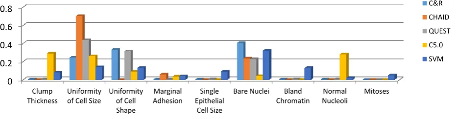
Table 5 shows the numerical illustration of the importance of the attributes with respect to five models C&R, CHAID, QUEST, C5.0, and SVM. It illustrates Bari Nuclei is the most important attribute in the C&R DT model; but it is less in importance for all the other models. Both CHAID and QUEST models are selected the attribute Uniformity of Cell Size as the most important attribute to make a decision. While the Clump Thickness attribute is attracting the importance with respect to the model C5.0. Clearly that the C&R DT model uses only 8 attributes; Clump Thickness, Uniformity of Cell Size, Uniformity of Cell Shape, Marginal Adhesion, Single Epithelial Cell Size, Bare Nuclei, Bland Chromatin, and Normal Nucleoli.
On the other side, CHAID uses only 3 attributes, which they are Uniformity of Cell Size, Marginal Adhesion, and Bare Nuclei. The QUEST model select 8 attributes similar to C&R model but they are different in the importance, which it is herein QUEST
named Uniformity of Cell Size; but in C&R is Bare Nuclei. The model C5.0 DT chooses the attribute Clump Thickness as more importance of the small difference with the second place (Normal Nucleoli) in the six attributes chosen, which they are Uniformity of Cell Size, Uniformity of Cell Shape, Marginal Adhesion, and Bare Nuclei respectively. Finally, SVM presents Bare Nuclei as more important attribute then, Uniformity of Cell Size and Bland Chromatin.
Table 5. The importance of attributes related to the five models
Nodes Importance
C&R CHAID QUEST C5.0 SVM Clump Thickness 0.0035 --- 0.004 0.292 0.08 Uniformity of Cell Size 0.2447 0.7041 0.4382 0.26 0.14 Uniformity of Cell Shape 0.3322 --- 0.3141 0.090 0.13 Marginal Adhesion 0.0035 0.0599 0.004 0.035 0.04 Single Epithelial Cell Size 0.0035 --- 0.004 --- 0.09 Bare Nuclei 0.4054 0.2361 0.2279 0.042 0.32 Bland Chromatin 0.0035 --- 0.004 --- 0.13 Normal Nucleoli 0.0035 --- 0.004 0.281 0.02 Mitoses --- --- --- --- 0.05
[image:8.595.77.543.626.748.2]Furthermore, Figure 5 illustrates that only 8 attributes are required to predict the diagnosis with this degree of accuracy by C&R, also only 3 attributes required in CHAID, and another degree of accuracy for QUEST needs only 8. Finally, only 6 attributes are required to predict the diagnosis with this degree of accuracy by C5.0 and all attributes have an accuracy ratio for SVM.
Fig.5. Most attributes important in the 10 trials using C&R, CHAID, QUEST, C5.0, and SVM with training subset.
0 0.2 0.4 0.6 0.8
Clump Thickness
Uniformity of Cell Size
Uniformity of Cell Shape
Marginal Adhesion
Single Epithelial
Cell Size
Bare Nuclei Bland Chromatin
Normal Nucleoli
Mitoses
C&R
CHAID
QUEST
C5.0
This figure shows that the relative importance of each attribute in the five classifier models C&R, CHAID, QUEST, C5.0 and SVM respectively represented by bars in different colors. The attribute Uniformity of Cell Size is appearing in this figure as completely more important attribute than others when applying the CHAID decision tree model, and followed by QUEST. Depending on this figure, the medical scientists can take a first impression about diagnose based on Uniformity of Cell Size attribute, then Bari Nuclei attribute.
[image:9.595.63.539.168.278.2]The table 5 and Figure 5 are given that the attribute Mitoses is not completely important with respect to other attributes. Figure 6 shows the cumulative charts of the five models for training and test subsets. The higher lines indicate better models, especially on the left side of the chart. The five curves are identical to test subset and almost identical to the training one. This figure shows that C5.0 line is the best in the training subsets; but in the testing subset the success is observed in CHAID.
Fig.6. The cumulative gains charts of the five models for training and test subsets.
The predictions of all models are compared to the original classes to identify the values of true positives, true negatives, false positives and false negative. These values have been computed to construct the confusion matrix as tabulated in
[image:9.595.119.477.375.535.2]table 6 where each cell contains the raw number of cases classified for the corresponding combination of desired and actual classifier outputs.
Table 6. The confusion matrices of decision tree and SVM models for training and testing subsets
Model Training Data Testing Data
Desired output Benign Malignant Desired output Benign Malignant C&R Benign 337= TP 7 =FP Benign 108 =TP 6 =FP
Malignant 11 =FN 136 =TN Malignant 3 =FN 91 =TN
CHAID Benign 330 14 Benign 107 7
Malignant 5 142 Malignant 1 93
QUEST Benign
331 13 Benign 107 7
Malignant 7 140 Malignant 2 92
C5.0 Benign
337 7 Benign 109 5
Malignant 3 144 Malignant 2 92
SVM Benign
343 1 Benign 109 5
Malignant 0 147 Malignant 2 92
[image:9.595.48.294.648.766.2]The values of the statistical parameters (sensitivity, specificity and total classification accuracy) of the four models were computed and presented in Table 7. Accuracy, Sensitivity and Specificity approximates the probability of the positive and negative labels being true. They assess the usefulness of the algorithm on a single model.
Table 7. Percentages of the statistical measures of C&R, CHAID, QUEST, C5.0, and SVM for training and testing
subsets
Model Partition Accuracy Sensitivity Specificity C&R Training 96.334 % 96.839 % 95.105 %
Testing 95.673% 97.297% 93.814%
CHAID Training 96.130% 98.507% 91.026% Testing 96.154% 99.074% 93.000%
QUEST Training 95.927% 97.929% 91.503% Testing 95.673% 98.165% 92.929%
C5.0 Training 97.963% 99.118% 95.364% Testing 96.635% 98.198% 94.845%
SVM Training 99.976% 100% 99.324% Testing 96.635% 98.198% 94.845%
The results in table 7, shows that the sensitivity, specificity and classification accuracy of all models have achieved 99.074% success of test samples. For CHAID model the accuracy is 96.130% of training samples and 96.154% of testing samples. However, the classification accuracy of the C&R DT model is 96.334% of training samples and 95.673% of testing samples. While 95.927% is the accuracy for QUEST of training samples, it is reduced to 95.673% of testing samples. In C5.0, the classification accuracy is 97.963% of training samples, and 96.635% of test samples; but the accuracy for SVM in training and testing are 99.976%, and 96.635%, respectively. Therefore, C5.0 is the best in accuracy for testing samples; but the best accuracy in training samples presented by SVM.
99.074% of testing samples. The 97.929% is the QUEST, classification sensitivity of training samples, but it is reduced to 98.165% of testing samples. Finally, the sensitivity of the C5.0 DT model is 99.118% of training samples, and 98.198% of testing samples. In the same context, SVM gives 100% and 98.198% for sensitivity analysis of training and testing samples, respectively. From the previous, SVM is the best in accuracy for training, but the CHAID is the best for sensitivity of testing samples.
Specificity is measuring the proportion of negatives which are correctly identified (e.g. The percentage of healthy people who
are correctly identified as not having the condition). In the QUEST model, the specificity is 91.503% of training samples, while the testing samples have specificity 92.929%. Last, but not least, in SVM the specificity 99.324% of training samples and 94.845% of testing samples at the same by C5.0.
In the same trend, the best in specificity is SVM of training and it is sharing C5.0 in testing samples. Figure 7 shows that the comparison of accuracy, sensitivity, and specificity with respect to the four models of decision tree, C&R, CHAID, QUEST, and C5.0 with SVM.
Fig.7. The comparison between C&R, CHAID, QUEST, C5.0, and SVM in accuracy, sensitivity, specificity
6.
CONCLUSION
Various data mining techniques are available in medical diagnosis, where the objective of these techniques is to assign patients to either a ‘healthy’ group that does not have a certain disease or a ‘sick’ group that has strong evidence of having that disease. Data mining have proved the ability to reduce the number of false positives and false negative decisions. Decision tree and SVM are the most popular and effective data mining methods. DT provides a pathway to find “rules” that could be evaluated for separating the input samples into one of several groups without having to express the functional relationship directly. They avoid the limitations of the parametric models and are well suited for the analysis of nonlinear events. This paper evaluated the classification performance of four different decision tree models CHAID, C&R, QUEST, C5.0, and comparing the results with SVM on the diagnosis of breast cancer using cytologically proven tumor dataset. The objective is to classify a tumor as either benign or malignant based on cell descriptions gathered by microscopic examination. The classification performances of the five models are evaluated and compared to each other using three statistical measures; Classification accuracy, sensitivity and specificity. This dataset has partitioned into training and test by the ratio 70%:30% respectively. Experimental results show that the effectiveness of all models. RBF-SVM identified a set of all attributes that are sufficient to achieve 100% classification sensitivity on training and sharing C5.0 in test subsets of 98.198%. However, SVM has achieved slightly better performance than the other. Importance analysis has shown that attribute "Uniformity of cell size" in CHAID DT and QUEST has achieved the most important attribute differentiating the cancerous from the healthy samples. While attribute "Bar Nuclei" proved importance with C&R, and SVM; but Clump Thickness attribute came in importance position by C5.0. Finally, RBF-SVM and DT models can be effectively used for breast cancer diagnosis to help physicians and oncologists. However, C5.0 DT uses fewer attributes than those required by RBF-SVM to predict the required class labels.
7.
REFERENCES
[1]Biggs, D., B. De Ville, and E. Suen. A method of choosing multi-way partitions for classification and decision trees. Journal of Applied Statistics, 18 (1), 49-62, 1991.
[2]Breiman, L., Friedman, J.H., Olshen, R.A., and Stone, C.J. Classification and Regression Trees, Belmont, California: Wadsworth, Inc, 1998.
[3]Buzdar. A. U. and R. S. Freedman. Breast Cancer. The 2nd edition, Springer Science and Business Media, 2008.
[4]C. Cortes and V. Vapnik. Support-vector networks. Machine Learning, 20(2), 273–297, 1995.
[5]Calle. J. Breast cancer facts and figures 2003–2004. American Cancer Society 2004. http://www.cancer.org/ (last accessed: Jan.2010).
[6]Duda and D.G. Stock pattern classification. John Wiley & Sons New York, 2001.
[7]F. Friedrichs and C. Igel. Trends in Neurocomputing. The 12th European Symposium on Artificial Neural Networks 64:107–117, 2005.
[8]Floares. A., A. Birlutiu. “Decision Tree Models for Developing Molecular Classifiers for Cancer Diagnosis”. WCCI 2012 IEEE World Congress on Computational Intelligence June, 10-15, 2012- Brisbane, Australia.
[9]H. Frohlich and A. Zell. Efficient parameter selection for support vector machines. IEEE International Joint Conference on Neural Networks, 3:1431–1436¸2005.
[10]Han. J. W. and M. Kamber. Data mining concepts and techniques, The 2nd edition, Morgan Kaufmann Publishers, San Francisco, CA, 2006.
[11]Hornik. K., Stinchcombe and H. White. Universal approximation of an unknown mapping and its derivatives using multilayer feedforward network. Neural Networks, 3, 359-66, 1990.
85.00% 90.00% 95.00% 100.00%
Training Testing Training Testing Training Testing Training Testing Training Testing
C&R CHAID QUEST C5.0 SVM
Accuracy
Sensitivity
[12]Hany A. Elsalamony.,Alaa M. Elsayad. Bank Direct Marketing Based on Neural Network and C5. 0 Models. International Journal of Engineering and Advanced Technology (IJEAT), ISSN: 2249 – 8958, Volume-2, Issue-6, August 2013.
[13]http://www.archive.ics.uci.edu/ml/index.html (last accessed: November 2012).
[14]http://www.komen.org/bci/bhealth/QA/q/and/a.asp (last accessed: Jan.2010).
[15]http://www.rulequest.com/see5/info.html (last accessed: November 2012).
[16]Karabatak. M. and M. Cevdet. An expert system for detection of breast cancer based on association rules and neural network. Expert Systems with Applications 36: 3465–3469, 2009.
[17]Kass, G. V. An exploratory technique for investigating large quantities of categorical data. Applied Statistics, 29 (2), 119-127, 1980.
[18]Kovalerchuc. B., E. Triantaphyllou, J. F. Ruiz and J. Clayton. Fuzzy logic in computer-aided breast-cancer diagnosis: Analysis of lobulation. Artificial Intelligence in Medicine, 11: 75–85, 1997.
[19]Lavanya. D., K. Usha Rani. “Ensemble Decision Making System for Breast Cancer Data”. International Journal of Computer Applications (0975 – 8887) Volume 51– No.17, August 2012.
[20]Lim, T.-S., Loh, W.-Y., and Shih, Y.-S. A comparison of prediction accuracy, complexity, and training time of
thirty-three old and new classification algorithms, Machine Learning Journal, vol. 40, 203-228, 2000.
[21]Loh, W.-Y. and Shih, Y.-S. “Split selection methods for classification trees”, Statistica Sinica, vol. 7, 815-840, 1997.
[22]N. Cristianini and J. S. Taylor. An introduction to support vector machines and other Kernel-based learning methods. Cambridge University Press, London, 2000.
[23]Nisbet. R., J. Elder and G. Miner. Handbook of statistical analysis and data mining applications. Academic Press, Burlington, MA, 2009.
[24]Pendharkar. P. C., J. A. Rodger, G. J. Yaverbaum, N. Herman and M. Benner. Association’s statistical, mathematical and neural approaches for mining breast cancer patterns. Expert Systems with Applications, 17:223–232, 1999.
[25]Ripley, B. D. Pattern recognition and neural networks. Cambridge University Press, Cambridge, UK, 1996.
[26]Su-lin PANG, Ji-zhang GONG, C5.0 Classification Algorithm and Application on Individual Credit Evaluation of Banks, Systems Engineering - Theory & Practice, Volume 29, Issue 12, Pages 94–104, December 2009.
[27]Ture. M., F. Tokatli and I. Kurt. Using Kaplan–Meier analysis together with decision tree methods (C&RT, CHAID, QUEST, C4.5 and ID3) in determining recurrence-free survival of breast cancer patients. Expert Systems with Applications, 36, 2017–2026, 2009.