30
Resolution of Inverse Problems for Electromagnetic
Levitated and Guided Systems using the Finite Element
Method and the Genetic Algorithms
Rima Delimi
L.E.C Laboratory, department
of electrotechnics, faculty of Engineering, University of
Constantine. Algeria
M.H Latreche
L.E.C Laboratory, departmentof electrotechnics, faculty of Engineering, University of
Constantine. Algeria
ABSTRACT
In an inverse problem, we are asked to find those values of the source that would give us a required performance. In this paper a technique based on the use of finite element method (FEM) and the genetic algorithms method (GA) in the solution of the inverse problem of an electromagnetic levitated and guided system is investigated, for that an inverse calculation of the current excitation was realized to have a constant levitation force.
Keywords
Inverse problems, Finite element method, Genetic algorithms, Magnetic levitation force.
1.
INTRODUCTION
The magnetic levitation domain is constantly in developing until their apparition, because of theirs many advantages, transport Vehicles are one of theirs most applications, were the electromagnetic levitated and guided systems offers the advantage of a very silent motion and of a reduced maintenance of the rail [1]. This paper shows a simple magnetic model for the study of the levitation and guidance forces produced by an electromagnet coupled with an iron rail, our goal is to keep the levitation force constant to ensure the stability of the system by calculating the needed current excitation, so we are asked to solve an inverse problem, for that, we propose the use of GA and FEM in the solution of the inverse problem of this system. That is, for a desired levitation force, we are asked to find the required excitation current (the rail shape taken into consideration in this paper).
The inverse problem related to the identification of the excitation current can be represented as the minimization of the error gained from the difference
between the magnetic force calculated by the Maxwell stress tensor method and the desired magnetic force.
The minimization procedure used in the simulation is based on the genetic algorithms. The use of the genetic algorithms is motivated by the simple reason that genetic algorithms only need to evaluate the objective function (error functional) to guide its search [2].
2.
THE
MAGNETIC
LEVITATION
FORCE EXPRESSION
The global force acting on the object is calculated by the integration of the Maxwell stress tensor on an arbitrary
closed surface S+ enclosing the domain of interest. The force evaluated by Maxwell stress tensor is well known by the next formula [3]:
dSS BnHt Bn Ht
n t
F 2
0 2
0 1
2 1
.
(1)
The accuracy of this method depends on the choice of the integral surface S+ and the accuracy of the normal component of the magnetic induction
B
n and the tangential component of the magnetic fieldHt.3.
APPLICATION
3.1
Device Description
The calculation we will do next use the dimensions of the electromagnet used in [4], here are the main values:
Fig1: Geometry model (Flat narrow rail)
Around the iron core there are two windings with 187 turns; the two windings are in a series connection. In these conditions by feeding the coils with the nominal current of 40 Amp the electromagnet will keep the nominal airgap to reach the nominal levitation force of about 2746.8N (240 Kg).
3.2
Electromagnetic Field Calculation
Maxwell's equation for the two dimensional magnetostatic problem was written as follows [5]:A = 0
A = 0
55 mm
80 mm 55 mm
20 mm
55 mm
55 mm 110 mm 220 mm
I= 40 Amp
A B
C D
31 s J )) ( 1
( r ot A
r ot (2)
x y y B xB A A
B , , (3)
With A the magnetic vector potential,
is the relative magnetic permeability, ands
J the current excitation density.
The potential vector distribution is obtained by solving the previous equation with the finite element method using the Matlab code.
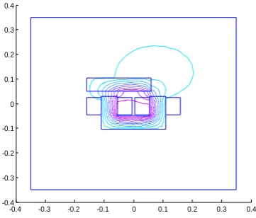
The next figure shows the computed field distribution.
-0.4 -0.3 -0.2 -0.1 0 0.1 0.2 0.3 0.4
[image:2.595.345.504.75.231.2]-0.4 -0.3 -0.2 -0.1 0 0.1 0.2 0.3 0.4
Fig 2: Magnetic vector potential distribution
In magnetic force calculation using the finite element method (FEM), the tangential and the normal force both depend on the tangential component of magnetic field Ht and the normal component of magnetic inductionBn.
Aproblem associated with the discretisation necessary in FE method is the inevitable introduction of discontinuities in field quantities which should be continuous. If the magnetic scalar potential formulation is used, the normal magnetic inductionBnwill not be continuous across the surface between elements, and if the magnetic vector potential formulation is used, the tangential field
t
H will not be continuous.
When determining the force density distribution on an air-iron interface, one has to evaluate the force on the common borders of two finite elements and the user is faced with the problem of which value of BnorHt to choose, in [6] suggested an approach using the magnetic vector potential formulation, which involved a weighted average of the air and iron tangential components of the magnetic field intensity. The Fig.3 shows the distribution of the normal component of the magnetic induction Bnalong the contour ABCDA in outer and inner finite elements with common borders.
0 5 10 15 20 25 30 35 40
-0.4 -0.3 -0.2 -0.1 0 0.1 0.2 0.3 0.4 Contour ABCDA N o rm a l c o m p o n e n t o f m a g n e ti c i n d u c ti o n ( te s la )
Normal induction density (Bn) in intern and extern elements
[image:2.595.76.257.225.379.2]Normal induction (Bn) in intern elements Normal induction (Bn) in extern elements
Fig 3: Normal magnetic induction (
B
n) in outer and inner elementsThe Fig.4 shows the distribution of the tangential component of the magnetic field density Htalong the contour ABCDA in outer and inner finite elements with common borders, and the average value between the two quantities.
0 5 10 15 20 25 30 35 40 -1
-0.5 0 0.5 1 1.5x 10
5 Contour ABCDA T a n g e n ti a l c o m p o n e n t o f m a g n e ti c f ie ld ( A m p /m )
Tangential field density (Ht) in intern and extern elements
[image:2.595.330.517.336.500.2]Tangential field (Ht) in intern elements Tangential field (Ht) in extern elements Average value of magnetic field
Fig 4: Tangential magnetic field (
H
t) in outer and inner elements and the average value3.3
The Magnetic Force Calculation
The Fig.5 shows the Modules of levitation force (Fy) and
guidance force (Fx) with a flat narrow rail depend on the displacement of the electromagnet with x.
-0.050 -0.04 -0.03 -0.02 -0.01 0 0.01 0.02 0.03 0.04 0.05
500 1000 1500 2000 2500 3000 3500
Displacement x (m)
M a g n e ti c f o rc e ( N )
Variation of levitation and guidance force with displacement
32
Fig 5: Modules of levitation and guidance forces with a flat narrow rail
We can notice that the levitation force is maximum when the electromagnet is centred (x = 0), whereas the guidance
force is zero. The more the electromagnet is far from the central position; the lower is the levitation force,
whereas the higher is the guidance force.
4.
RESOLUTION OF THE INVERSE
PROBLEM
To show the rail shape influence, the inverse problem will be calculated for two rail shapes (Flat narrow rail, and C-shaped rail); the next figure shows the computed field distribution for the second rail shape.
-0.4 -0.3 -0.2 -0.1 0 0.1 0.2 0.3 0.4 -0.4
-0.3 -0.2 -0.1 0 0.1 0.2 0.3 0.4
Fig6: Geometry model (C-shaped rail) It is clear that the direct calculation doesn‟t take into account all the features of the real application.
Even in the case of no disturbance the electromagnet have to support a constant vertical force due to the weight of vehicle. As the electromagnets are the actuators of a levitation system that aims to hold a constant vertical position (e), they must provide constant levitation force .The problem is how to calculate the module of guidance force (Fx) and current excitation to keep a constant levitation force (Fy) for each position of the electromagnet, for that we must solve the inverse problem in order to find an effective solution concerning the current excitation and the guidance force (Fx) generating a desired magnetic force (Fy).
4.1
Inverse Problem
To resolve the inverse problem of an electromagnetic device, the most operational definition consists in determining causes (parameters) knowing effects (started from its evolution).It is the inverse of that called direct problem [7, 8].
Fig7: Direct and inverse Problems
Inverse problem to be analyzed to find the current excitation is as follows:
Find I giving Fc (I) =Fd (4)
Where: Fd is the desired magnetic levitation force. Fc is the calculated magnetic levitation force.
In order to solve the inverse problem, it is necessary to the first time to formulate it in the form of minimization of an objective function of error between real measurements
(desired) and synthetic measurements (the solution of the direct problem). In this study, the adopted error
function to minimize is the least squares:
2
2 1 )
(
Fd Fc Fd parameters
error (5)
The algorithm of resolution is: the Genetic Algorithms method, associated to the finite element method.
4.2
Diagram of the Genetic Algorithms
Method
The steps of GA method are illustrated in the next diagram [9, 10]:
Fig8: diagram of the GA method
4.3
Results
The minimizing procedure used in the simulation is based on the genetic algorithms. The GA begins by randomly generating a population of 100 strings.
4.3.1
First shape
We first consider a flat narrow rail coupled with the electromagnet in an offset position (0.05 m at left).
Next figure shows the convergnece of the algorithm for a desired magnetic levitation force Fd= 2746.8N which calculated for the same system in [4]. After 50 generation, excitation current obtained is I=52A and the corresponding guidance force is Fx=765.18N.
Start
Initialization (Initial Population)
Resolution of the magnetic equation for each individual of the population
Calculation of the magnetic force
Fitness calculation
error evaluation
Convergence Selection and reproduction
End
input output
Direct problem
33 0 10 20 30 40 50 60 70 80 90 100
0 0.1 0.2 0.3 0.4 0.5 0.6 0.7 0.8 0.9
1x 10 -3
Generations
E
rr
o
r
Fig9: Convergence of the genetic algorithm (Flat rail)
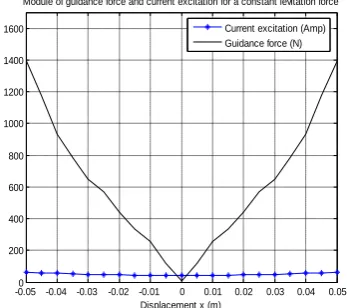
In Fig.10 we show the result for the flat rail: the guidance force and the current needed to provide the guidance force for different position of the electromagnet (displacement with x).
-0.050 -0.04 -0.03 -0.02 -0.01 0 0.01 0.02 0.03 0.04 0.05
100 200 300 400 500 600 700 800 900
Displacement x (m)
Module of guidance force and current excitation for a constant levitation force
[image:4.595.341.515.342.496.2]Current excitation (Amp) Guidance force (N)
Fig 10: Module of guidance force and current for a constant levitation force operating with a flat narrow rail
4.3.2
Second shape
Now we consider a C-shaped rail coupled with the electromagnet in an offset position (0.05 m at left).
Next figure shows the convergnece of the algorithm for a desired magnetic levitation force Fd= 2550.6N which calculated for the same system in [4]. After 45 generation, excitation current obtained is I=62 A and the corresponding guidance force is Fx=1393N.
0 10 20 30 40 50 60 70 80 90 100
0 0.2 0.4 0.6 0.8 1 1.2 1.4x 10
-3
Generations
E
rr
o
r
Fig11: Convergence of the genetic algorithm (C-shaped rail)
In Fig.12 we show the result of the C-shaped rail: again the guidance force and the current needed to provide the guidance force for different position of the electromagnet (displacement with x).
-0.050 -0.04 -0.03 -0.02 -0.01 0 0.01 0.02 0.03 0.04 0.05
200 400 600 800 1000 1200 1400 1600
Displacement x (m)
Module of guidance force and current excitation for a constant levitation force
Current excitation (Amp) Guidance force (N)
Fig12: Module of guidance force and current for a constant levitation force operating with a C-shaped rail
In the inverse calculation the C-shaped rail is better than the flat rail; it can give with the same electromagnet twice the guidance force as the flat rail (a big guidance force able to keep the electromagnet centred).
4.3.3
Changing the value of the airgap
The inverse calculations of the levitation characteristic represented in the previous paragraph for the two types of rail have been obtained with a 20 mm airgap. How does the characteristic change if we keep a constant levitation force and we change the airgap?
We will only consider the case of the coupling of the electromagnet with a C-shaped rail. In Fig.13 and
34
-0.05 -0.04 -0.03 -0.02 -0.01 0 0.01 0.02 0.03 0.04 0.05
10 20 30 40 50 60 70 80
Displacement x (m)
Module of current excitation for a constant levitation force
C
u
rr
e
n
t
e
x
c
it
a
ti
o
n
(
A
m
p
)
Airgap e = 20 mm Airgap e = 15 mm Airgap e = 10 mm Airgap e = 5 mm
Fig13: Module of current excitation for a constant levitation force operating at different airgap values
(C-shaped rail)
-0.050 -0.04 -0.03 -0.02 -0.01 0 0.01 0.02 0.03 0.04 0.05 200
400 600 800 1000 1200 1400 1600 1800
Displacement x (m)
M
a
g
n
e
ti
c
f
o
rc
e
(
N
)
Module of guidance force for a constant levitation force
Airgap e = 20 mm Airgap e = 15 mm Airgap e = 10 mm Airgap e = 5 mm
Fig14: Module of guidance force for a constant levitation force operating at different airgap values (C-shaped rail)
A smaller airgap results is a weaker guidance force. We can notice that the slope of the curves for x=0 is always the same for different airgaps.
We can notice that the guidance force is higher than in the previous evaluations.
The inverse calculation result evidence the better guidance force obtained with a C-shaped rail.
5.
CONCLUSION
Resolve an inverse problem, is the question to determinate the descriptive magnitudes of the device which satisfy to a definite functioning conditions.
In this paper, for the study of the levitation and guidance forces produced by an electromagnet coupled with an iron rail, an inverse calculation of current excitation was realized
to have a definite force levitation value (Inverse calculation gives current excitation values able to keep the levitation force constant), for that, the use of the finite element method associated to the genetic algorithms method in the resolution of this inverse problem is investigated. Results of simulation show the feasibility and the effectiveness of the approach suggested after a few iterations.
6.
REFERENCES
[1] J.Delamare,"Suspensions magnétiques partiellement passives "Thése de Doctorat soutenue au LEG Grenoble, France, 1994.
[2] Y.J. Favennec, “Modélisation numérique en chauffage par induction. Analyse inverse et optimisation”, thèse de Doctorat, Paris, 2002.
[3] Olivier Barre, „‟Contribution à l‟étude des formulations de calcul de la force magnétiques en magnétostatique, approche numérique et validation expérimentale „‟, Thèse de Doctorat, Ecole centrale de Lille Université des sciences et technologies de Lille, 15 Décembre 2003. [4] D‟Arrigo Aldo, Rufer Alfred,"Design of an integrated
electromagnetic levitation and guidance system for Swiss Metro", Swiss Federal Institute of Technology, Industrial Electronics Laboratory, 1999.
[5] J. P. A. Bastos, N. Sadowski, "Electromagnetic modeling by finite element methods", Library of Congress Cataloging-in-Publication Data, New York, USA, 2003.
[6] A. Benhama, A.C. WiIIiamson, A.B.J. Reece," Virtual work approach to the computation of magnetic force distribution from finite element field solutions", IEE Proc-Electr. Power Appl., Vol. 147, No. 6. November 2000.
[7] Y. Lefèvre, F. Messine, J. Fontchastagner et X. T. H. BUI, „‟ Association de différentes méthodes optimisation et de modèles de calcul du champ magnétique „‟, dans Electro-technique du Futur – EF‟2007, Toulouse, Sept. 6-7- 2007
[8] Julien FONTCHASTAGNER, „‟ Résolution du problème inverse de conception d‟actionneurs électromagnétiques par association de méthodes déterministes d‟optimisation globale avec des modèles analytiques et numériques‟‟, Thèse de Doctorat, Université de Toulouse, 2007. [9] L. Saludjian , J.L. Coulombi , “ Genetic algorithm and
Taylor development of Finite Element solution for shape optimization of electromagnetic devices ”, IEEE Trans. On Magnetics, vol. 34, n°5, Sept.1998, pp.2841-2844. [10]O. Hajji, S. Brisset, P. Brochet, “ A stop criterion to
accelerate magnetic optimization process using genetic algorithms and Finite Element analysis ”, IEEE Trans. On Magnetics, vol. 39, n°3, May.2003, pp.1297-1300.