Quantum Field Theory of Graphene with Dynamical Partial Symmetry Breaking

(1)

http://dx.doi.org/10.4236/jmp.2014.510100

Quantum Field Theory of Graphene with

Dynamical Partial Symmetry Breaking

Halina V. Grushevskaya, George Krylov

Physics Department, Belarusian State University, Minsk, Belarus Email: grushevskaja@bsu.by

Received 17 April 2014; revised 14 May 2014; accepted 11 June 2014

This work is licensed under the Creative Commons Attribution International License (CC BY). http://creativecommons.org/licenses/by/4.0/

Abstract

The quantum field theory approach has been proposed for the description of graphene electronic properties. It generalizes massless Dirac fermion model and is based on the Dirac-Hartree-Fock self-consistent field approximation and assumption on antiferromagnetic ordering of graphene lattice. The developed approach allows asymmetric charged carriers in single layer graphene with partially degenerated Dirac cones.

Keywords

Graphene, Asymmetric Charged Carriers, Dirac-Hartree-Fock Self-Consistent Field Approximation

1. Introduction

The ongoing boom in experimental researches of graphene is not accompanied, however, by substantial devel-opment of nanoelectronic components using its unique properties. The one of the possible reasons of this situa-tion could be the absence of satisfactory descripsitua-tion of its electrophysical properties on the basis of quantum field theory.

The ab initio calculations by muffin-tin orbital method and usage of random phase approximation (RPA) for polarization operator to investigate the balance of exchange and correlation interactions on band structure of loosely-packed crystals have shown that strong exchange leads to appearance of an energy gap in the spectrum [1]. Conversely, strong correlation interaction leads to tightening the gap in the band spectrum. The spin non- polarized ab initio simulations of partial electron densities of two-dimensional graphite have shown that the ma-terial is a semiconductor. Interlayer correlations tighten energy gap that results in semi-metal behaviour of three- dimensional graphite [1]. The presence of a gap in band spectrum of graphene (at Dirac points K K, ′) would increase theoretical estimation of its conductivity to _{πe h}2

(2)

(minimal) conductivity of monolayer graphene [3]-[5] with its experimental value _{4e h}2

[6]-[12].

Energy gap ~10 meV can be in spectra of nanostructures with photon-dressed ground state [13]. With mea-surement accuracy ~1 meV, permissible at the present level of technological development, the gap is not regis-tered [14], though a sharp change of the Fermi velocity vF in Dirac point K K

( )

′ , described in Hartree-Fock and RPA [14], as well as when using the ab initio simulations [15] is the experimental fact [14].

Quantum field theory [16] of pseudo-Dirac quasiparticles [17]-[20] in RPA gives a strong screening which destroys the excitonic pairing instability if dynamic fermion mass mq is small in comparison with chemical potential µ: mq ≤µ. The existence of dynamic screening for this system with physical flavor N=2, calcu-lated by Eliashberg self-consistent technique, makes the value of mq non-zero for momentums

6

10

q < − [16]. Unfortunately, such a range of values of q also gives practically vanishing mass mk_F q vF 10 12

−

<

 for the

Fermi momentum kF and Fermi velocity

6

10 m/s F

v  . Additional possible lack of this approach is that though pseudo-Dirac fermions act in 2 + 1 dimensional space-time, an electromagnetic field is defined as usual in 3 + 1 dimensions [2] [16] [21] (otherwise Coulomb interaction in 2D space would be log r rather than needed 1/r).

In papers [22]-[24] one uses a known analogy between the mass of a particle in the kinetic energy and a factor entered as the mass tensor mij in a quadratic term in the energy expansion of a single-particle state; the mag-neto-transport term for which there is no such an analogy is discarded. Such description of particles collisions in impurity-free (pure) graphene as electron-phonon scattering gives an estimate of the dynamic conductivity

( )

2

πe 2h at low temperature T→0 [22]-[24].

In the reference frame where a fermion with nonzero rest mass moves with a velocity v, its bispinor wave function Ψ

( )

t = Ψ

{

_σup

( )

t ,Ψ_σdown

( )

t

}

in addition to non-zero upper components Ψup_σ

( )

t acquires non-zero lower (“positron”) components Ψ_σdown

( )

t [25] [26]

( )

(

)

1 2

( )

(

)

1 2 1 2 2

1 1

cosh 1 e , cosh 1 e ,cosh 1 .

2 2

up i t down i t

p p

t t v c

p

ε ε

σ χ − ψ σ χ − ψ −χ

⋅

Ψ = + Ψ = σ p − = − (1)

Changing the light speed c→vF in (1), the pseudo-spinor wave function Ψp

( )

t of quasiparticles in

gra-phene can be written as a sum of electron wave functions (1):

( )

₁

( )

(

( )

)

† ₁

(

)

(

)

e 1 e 1

2 2

p p

i t i t

up down up down

p t t t t t p p p

ε ε

σ σ σ σ

− − −

  _ _

Ψ = _Ψ + Ψ + Ψ + Ψ _ _ + ⋅ + − ⋅ _Ψ

  σ p σ p (2)

where ε =p v pF . Due to the process of electron-hole pairs’ production, the current j [27] oscillates [28]

( )

† †

(

)

†

(

)

2

0 1 1, 0 2 , 1 2 e

2

p i t F

F p p p p

p p

p ev i

t ev

p

p p

ε

⋅  ⋅ 

= + + = Ψ Ψ = Ψ _ − + × _Ψ

 

∑

p

∑

p p

j j j j j σ j σ σ σ p (3)

where oscillating summands † 1, 1

j j are called “Zitterbewegung” terms. Drawback of pseudo-electrodynamics of graphene [28] is the divergence of the expression (2) at v→vF.

Weak localization of states can be introduced through non-zero spin-orbit interaction. A possibility of the ab-sence of inversion center for spin-polarized electron density of monolayer grapheme, related with this fact pos-sibility of non-zero spin-orbit contribution G I,

SO

(3)

de-scribed via the appearance of a gap stipulated by excitonic pairing mechanism and with a value of the same or-der of magnitude as the aforementioned (induced) one. Besides, the Hall effect is accompanied by intensive process of electron-hole symmetric pair production in the form of “Zitterbewegung” for wave functions [3] [27] [37]. This demonstrates that the “Zitterbewegung” phenomena and the gap of nanostructures with photon- dressed ground states are capable to neutralize resonant mechanism of the induced skew symmetry.

Electromagnetic interaction between N Dirac particles leads to a renormalization of their masses [38]. On the one hand, this dynamic (renormalized) mass mq of charged carriers in graphene should be sufficiently small: mq ≤µ, to be an agreement with experimental data. On the other hand, the value of mq should be finite that allows at least getting a match with the experimental value of the dynamic conductivity of graphene [2] [22].

The most promising is the use of Dirac-Hartree-Fock self-consistent field approximation for the description of spin-dependent electrical properties of graphene, since the estimate of dynamic mass of the quasiparticles in graphene in this approximation is given by  ₁₀ 8

AB BA c −

Σ Σ  [39].

Charged carrier asymmetry in graphene transport experimentally found in [40] [41] by a method [42], allows assuming non-coincidence of Dirac cone with its replica except for K K

( )

′ -point. In the paper [43], it has been shown that in the flavor model N=2 charged carriers are symmetric as well as the graphene band structure.

The goal of this paper is to construct a pseudo-bispinor description of graphene, which is based on the Dirac- Hartree-Fock self-consistent field approximation, and to propose a flavor model N =3 for the graphene with spin-polarized sublattices. Coulomb interaction in the model is dynamically screened not due to self-consistent motion of an electron with respect to a hole as in flavor models N =2, but due to self-consistent motion of negatively charged three-particle exciton state relative to positively charged three-particle exciton

(

N=3

)

.

The paper is organized as follows. In Sections 2 and 3 we shortly introduce the approach [39] and use it in a simple tight-binding approximation of the problem and massless case. Section 4 gives explicit expressions for exchange interaction matrices allowing further simulating quantities of interest, which are performed and dis-cussed in Sections 5 and 6; in Section 7 we summarize our findings.

2. The Equations of Self-Consistent Charged Carriers Motion in Graphene

In papers [39] [44]-[46] a new approach has been proposed to describe graphene electronic properties. It utilizes a quasi-relativistic Dirac-Hartree-Fock self-consistent field approximation and assumption on ferromagnetic or-dering of the sublattices A B, (with anti-ferromagnetic ordering of the lattice as a whole). In this approach the graphene is described by the following stationary equation for the second-quantized fermion field ˆ†

A

σ

χ− :

( )

( ) ( )

{

}

_ˆ†

( )

_ˆ†

( )

ˆ 1 0, 0, .

A A

qu x x

F rel _AB rel _BA qu

v c i i χ₋_σ σ E p χ₋_σ σ

⋅p − Σ Σ r − = r −

σ (4)

Here points K K

( )

′ in the Brillouin zone of monolayer graphene are designated as K_A

( )

K_B , p is the momentum operator, operator ˆqu

F

v is defined as

( )

(

)

ˆFqu xrel A B .

BA

v = Σ_ +cσ⋅ K +K _ (5)

(

σ σ σx, y, z

)

=

σ is the vector of Pauli matrices, 2D transformation matrices

( ) ( )

x , x rel _BA rel _AB

Σ Σ are determined

by an exchange interaction term x rel Σ

( )

† †

0

ˆ ˆ

0, 0, 0, 0, ,

ˆ ₀ ˆ

A A

B B

x rel

AB x

rel

x rel

BA

σ σ

χ χ

σ σ σ σ

χ χ

− −

 Σ 

  _ _ 

   

Σ _ _ − =_ __ _ −

Σ

  _ _ 

r r

r r (6)

( )

†

( )

†

( )

†

( ) (

)

( )

1

ˆ 0, d ˆ 0, 0, ˆ ˆ 0, ,

v

B A

B _i _i B

NN x

rel _AB i i i i i i

i

V

σ _σ _σ σ

χ σ χ σ σ χ₋ χ₋ σ_′

=

Σ r =

∑∫

r r − r r−r r − (7)

( )

†

( )

†

( )

†

( )

1

ˆ 0, d ˆ 0, 0, ˆ ( )ˆ 0, .

v

B

A A _A

i i

NN x

rel _BA i i i i i i

i

V r r

σ _σ σ σ

χ σ χ σ σ χ χ σ

′ ′

′ ′ ′ ′ ′

− ₋

′=

Σ r − =

∑∫

r r − r  − r (8)

Now, we perform the following non-unitary transformation of the wave function for graphene

†

_{( )}



0, 0, .

A A

x rel

BA

σ σ

χ− −σ = Σ χ− −σ (9)

(4)

pure two-dimensional case. After this transformation, Equation (4) takes the form similar to a pseudo-Dirac ap-proximation of two-dimensional graphene:



{

}

†

( )

†

( )

2 ˆ _A 0, ˆ _A 0, , 1

AB

D BA BA AB qu

cσ ⋅p − Σ Σ χ₋_σ r −σ =cE p χ₋_σ r −σ q (10) where BA AB

( ) ( )

relx xrel

BA AB

Σ Σ = − Σ Σ , 2

( )

2

( )

1

AB x x

D rel D rel

BA BA

−

= Σ Σ

σ σ , σ2D =

(

σ σx, y

)

,

( ) ( )

1

† †

ˆ ˆ

A A

x x

BAχ σ rel _BA rel _BAχ σ

− − = Σ Σ −

p  p  , E_qu=E v_{qu F}ˆ−1.

In a similar way we can write down the following stationary equation for the second quantized fermion field

†

ˆ B

σ

χ+ on the sublattice B:



_{( )}

†

_{( )}

†

_{( )}

2 ˆ B 0, ˆ B 0,

BA

D AB AB BA qu

c χ₊_σ σ cE p χ₊_σ σ

 ⋅ − Σ Σ  =

 σ p p  r   r (11)

where AB BA

( ) ( )

relx xrel

AB BA

Σ Σ = − Σ Σ , AB

( ) ( )

xrel relx 1

AB AB

−

= Σ Σ

p p , ˆ†

( )

0,

( )

ˆ†

( )

0,

B B

x rel

AB

σ σ

χ₊ r σ = Σ χ₊ r σ .

Due to the fact that

( ) ( )

Σxrel _BA≠ Σxrel _AB, the vector pBA of the Dirac cone is somehow rotated and stretched in respect to the vector pAB of its replica.

3. The Equation of Motion of Massless Charged Carriers in Graphene

Massless approximation of Equation (10) reads

( )

† †

2 ˆ B 0, ˆ B 0, . BA

D⋅pABχ+σ r −σ =Equ p χ+σ r −σ

σ (12)

Let wave functions φ_↑ and φ_↓ with spin up and down respectively has the form

1 2 0 1 1 , . 0 2 2 φ φ φ φ ↑ ↓     = _{ } = _{ }

    (13)

Bispinor wave functions of quasiparticles moving on the Dirac cones and its replicas can be represented as the free Dirac field of π (pz)-electrons:

( )

( ) ( )

(

)

( )

{

}

( )

{

}

( )

{ }

( )

{ }

( ) ( ) 1 † 2 † 2 1 exp

ˆ _0, _exp

e

,

ˆ _0, ₂ _exp

exp A B

A B A B

A B

A B A B

B A

B A _{B A}

B A k i k k k i i i i σ σ σ σ θ φ θ φ

χ σ χ

χ

χ σ _θ _φ

θ φ − − ⋅ − − + +  ₋       −   −     =   ≡          ₋ _ _          

K q r

r r   (14) ( ) 

_{( )}

( ) 

_{( )}

( ) ( )

(

)

( )

{ }

( )

{ }

( )

{

}

( )

{

}

( ) ( ) 2 † 1 † 1 2 exp exp 0, _e 2 0, exp exp A B

A B A B

A B

A B A B

B A

B A B A

B A k i k k k i i i i σ σ σ σ θ φ θ φ

χ σ χ

χ

χ σ θ φ

θ φ − − ⋅ + + − − ₋        _ _{ } _  ₌ _ _{ }_≡ _   _ _ _ _  −  _ − _ _ _     −    

K q r

r r (15) where

( )

( ) ( ) ( ) ( )

{

}

{ }

(

( )

)

3 2 1 exp

2π 2 i

A B l

A B A B

i i A B A B l n l

N

φ =

∑

_ −  _{ } − _ ψ −

R

K q R r r R (16)

is a Bloch function.

(5)

de-scribed by the Formulae (14), (15):

( )



( )



( )

† † † †

ˆ A _A , ˆ B _B for , .

i i

i i

σ σ

χ χ χ χ

′ −

− r ≡ r r ≡ r ∀ ′ (17)

Then, in this approximation we can write matrices

( )

relx AB AB

Σ ≈ Σ and

( )

relx BA BA

Σ ≈ Σ without self-action as

( )



_{( )}

₍

₎

_{( )}

(

)

( )

_{( )}

1 † * 1 * * 1

1 1 1 2 2

3 2 _* _*

1 ₂ ₁ ₂ ₂

0, d

e e e e e

1

d

2 e e e e _e

v

B B A B B

A A k

kA kB kA kB B

v

kA kB kA kB

N N x

rel AB i i i i

AB

i

i i i i

N N

i i i i

i i _i _i _i _i

i _i _i _i _i

V

σ σ σ σ σ

θ

θ θ θ θ

χ σ χ χ χ χ

φ φ φ φ φ

φ φ φ φ

− + − − + =   − − ⋅ − − − _ _ − − − − =  

Σ ≈ Σ = − _ ⋅ _

 _{ −}   = −    

∑ ∫

K q r

r r r r r r r

r r r r r

r r r

r r r r ( )

( )

1

, A A kB

i θ φ  − ⋅ −         

 K q r r 

(18)

( )



_{( )}

₍

₎

_{( )}

(

)

( )( )

( )

( )( )

( )

( ) 1 † * 1 * * 1

2 2 2 1

3 2 * *

1

1 2 1 1

0, d

e 1 e e e e

1

d

2 _e _{1 e} _e _e

v

A A B A A

A A k

kB kA kB kA A

v

kB kA kB kA

N N x

rel _BA BA i i i i

i

i i i i

N N

i i i i

i i i i i i

i

i i i i

V

σ σ σ σ σ

θ

θ θ θ θ

χ σ χ χ χ χ

φ φ φ φ

− − − + + − =  − − ⋅ − − − _ − − − =  

Σ − ≈ Σ = − _ ⋅ _

₋ ₋ ₋    = −  −   

∑ ∫

K q r

r r r r r r r

r r r r

r r r

r r r r

( )

_{( )}

1 2

. ei A A θkA

φ φ     −_ − ⋅ + _      

 K q r 

r r

(19)

It follows from the expressions (18), (19) that the matrices ΣAB and ΣBA have the form

( )

{

}

₍

_{) ( ) ( )}

( ) ( )

* *

1

1 1 1 2

* *

1 2 1 2 2

1

e d ,

2

v kA kB

N N

i _i _i _i _i

AB i i

i i i i i

V

θ θ φ φ φ φ

φ φ φ φ

− − −

=

 

Σ = −  

 

 

∑ ∫

r r r r

r r r

r r r r (20)

( )

{

}

₍

₎

( ) ( )

* *

1

2 2 2 1

* *

1 1 2 1 1

1

e d .

2

v kA kB

N N

i _i _i _i _i

BA i i

i i i i i

V

θ θ φ φ φ φ

φ φ φ φ

− − −

=

 − 

Σ = − ₋ 

 

 

∑ ∫

r r r r r r r

r r r r (21)

Let us find the matrices ΣAB and ΣBA in tight-binding approximation. To do it, we substitute the expres-sion (16) into matrices (20), (21) and calculate integrals entered in elements of these matrices, for example

(

) ( ) ( )

( )

(

)

{ }1

(

)

{ }2

(

{ }

)

* *

2 1 3 1

,

2

d d e .

2π

i i A A lA lA

A A

A A i

i i i i i i n i l n i l

l l

V V n

N

φ φ ′ ψ ψ

′ ′

 −  ⋅_ − _  

− = −

∑

− −

∫

K q R R

r r r r r r r r r R R (22)

Taking into account that the vector difference ri−r lays in i-th primitive cell:

2D i− = i

r r r , we transform (22) as

(

) ( ) ( )

( )

{

}

{ }1

(

)

{ }2

(

)

* 2 1

2 2 * 2 2

3

,

d

2

d exp

2π A A A A

A A

i i i i

D D i i D D

i i A A l l n i l n i l

l l V V i N φ φ ψ ψ ′ ′ ′ −     = _ − _{ }⋅ − _ − −

∫

∑

∫

r r r r r

r r K q R R r R r R (23)

where i-th primitive cell is obtained from the base one by a rotation on an angle

(

2i±1 60 ,

)

i=1, 2, 3; ( ) ( )

A A A A l _′ = l _′ −

R R r. Let us account for nearest neighbors only in (23):

(

) ( ) ( )

( )

{

}

( )

{ }1

(

)

{ }2

( )

* 2 * 2 2 2

2 1 3

1

d exp d .

2π

i D D D D

i i i i A i i i n i i n i i

V − φ φ = i_ − _⋅ V ψ − ψ

∫

r r r r r K q δ

∫

r r δ r r (24)

As a basic set we choose _{{ }} _{{ }}

2 , 1

n n

ψ ψ orbitals of π-electrons: _{{ }}

(

)

( )

2 1 pz i 2 pz ,

n c c

ψ = ψ r±δ + ψ r

∑

2i=₁ci2=1;

{ }n1 pz

( )

ψ =ψ r . Energy of an electron is not changed with rotation on a lattice vector. Therefore, we can use the symmetry of the problem for simulation simplification by choosing e.g., δ1 and q, as δi, qi.

4. Partially Broken Symmetry of Model

N

= 3

(6)

(

)

( )

{

}

( )

3

2 2 2

3

1

* * *

p 2 p , 2 p 2 p 2 p , 2

* * *

p , 2 p , 2 p 2 p , 2 p 2 p 2 p , 2

3

1

e exp d d d

2 2π 2

2 1

e 2 2π

kA kB

z z i z z z i

z i z i z i z z z i

i i

AB i i A i i D D D

i

D D D D D

D D _z D D D D D

q θ θ i z V x y

δ

ψ ψ ψ ψ ψ

ψ ψ ψ ψ ψ ψ ψ

− − = − − − − −  

Σ = _ − _⋅

 _ + _    ×_ _  +  _ +  _{ } + _     =

∑

K q

∫ ∫

r

r r r r r

r r r r r r r

δ δ

δ δ δ δ

δ

( ) 3

_{

_}

1

exp ,

kA kB

i _i _nd

A i i AB i

i

θ −θ

=

 − ⋅ Σ

 

∑

K q δ

(25)

(

)

( )

{

}

( )

3

2 2 2 3

1

* * *

p , 2 p 2 p 2 p , 2 p , 2 p , 2 p 2

* * *

p 2 p 2 p , 2 p 2 p , 2

1

e exp d d d

2 2π 1 2 2 1 2

kA kB

z i z z z i z i z i

z z z i z z i

i _i

BA i i A i i D D D

i

D D D D D D _z D

D D D D D

q θ θ i z V x y

δ

ψ ψ ψ ψ ψ ψ ψ

ψ ψ ψ ψ ψ

− − =

− −

 

Σ = _ − _⋅

 _ ₊ _{ } ₊ _ ₋ _ ₊ _        ×   − _ + _    =

∑

K q

∫ ∫

r

r r r r r r r

r r r r r

δ δ δ δ

δ δ δ

( )

{

}

3 3 1

e exp .

2π

kA kB

i _i _nd

A i i BA

i i

θ θ − −

=

 − ⋅ Σ

 

∑

K q δ

(26)

Here it was chosen the upper sign for π-orbital _{{ }}

2

n

ψ and was introduced the following notion

( )

(

)

p ,_z _i 2D p_z 2D i

ψ ±δ r =ψ r ±δ . Secular equation with this basic orthogonal set

{ }

i has the form

1 2 1 ˆ . ˆ BA

D AB F

j F

i i v j j E i E

i v i

ψ − ψ ψ

⋅p =

∑

=

σ (27)

Due to the fact that i v iˆ_F ∝v_F and the wave function is defined up to a phase multiplier, then Equation (27) is reduced to

2 . BA D AB F E v χ χ

⋅p =

σ (28)

Let us rewrite Equation (28) in momentum representation as

(

)

1

(

)

2 ,

p

p i AB i i D AB j j j AB p p p

i j F

E

q q q q

v

χ _Σ δ _Σ− δ χ ₌ χ χ

∑

σ p (29)

where qi+qj =0 owing to momentum conservation law. Then one can obtain 2

BA D

σ in an explicit form

(

)

( )

(

) (

)

(

) (

)

3 2 1 1 1

2 2 2 3

2 1 1 . 1 k k

BA nd nd k

D AB i i D AB j j AB D AB

k k

k i

q q

i

δ − δ − =

=

 ₋ _⋅ _{− ⋅} ₋ 

 

≡ Σ Σ = −Σ Σ

 ₊ _⋅ _{− ⋅} ₊   

∑

q q q q   δ δ

σ σ σ

δ δ (30)

Substituting known expressions for eigenfunctions of hydrogen-like atom [47] and evaluating integrals, we obtain rather lengthy

( )

q -dependent invertible matrices, for q=0 they are pure numeric and up to a common scalar prefactor read

( )

0.062 0.54

( )

0.42 0.045

, .

0.045 0.42 0.54 0.062

AB A BA A

−

   

Σ =_ _ Σ =_ _

−

   

K K (31)

The most interesting thing is that eigenvalue problem (28) gives precisely the known dispersion laws

( )

2 2

x y

E q = ± q +q , that is problem is persistent up to q3 variations.

Now, we take into account higher order in q terms when evaluating ΣAB,ΣBA. Dependence of the Fermi energy EF

( )

n on the surface carriers concentration n is the replacement of

(

A

)

F

(

F

)

F

(

π

)

E q K →E q k =E q n so that q2x+q2y =πn=kF2. The Fermi energies

( )

e F

(7)

( )

h F

E n for electrons and holes, respectively, are represented in Figure 1. One can see that the hole and electron bands are symmetric. Six mini-zones around points K K, ′ of Brillouin zone are also observable in Figure 1.

5. Asymmetrical Charged Carriers at Large Fermion Density

Now, let us show that the spectrum E q

( )

corresponding to Equation (12) can deviate from the conic form at large concentration n. According to Figure 1, for _n_₁₀14 _m−2

the Fermi level is in the region with unbroken symmetry of the Dirac cone. When _n_₁₀15 _m−2

, the Fermi level enters the region with broken symmetry of the Dirac cone. In this region, there is a Fermi energy curve EFe h( ) which has local hyperbolic points of a “sad-dle” type. Fermi curves passing through or near these hyperbolic points are local maxima and minima. Since in these points “trajectories” of quasi-particle motion (i.e., the configuration space of the system) are unstable, not all holes (electrons) can reach the Dirac cone (replicas) and annihilate. We demonstrate E q

( )

surface sections for few qx in Figure 2.

Figure 2(a) emphasizes that in the vicinity of Dirac point the cone is persistent due to symmetry (section crosses original cone and its replicas simultaneously), at higher values of q, higher order corrections start to contribute. An energy dispersion law for 2D graphene is linear near Dirac cone corner at µ=0 (see Figure 2(a)). When section crosses original cone only (Figure 2(b)), we find symmetrical section of the Dirac cone.

(a) (b)

Figure 1. Fermi energy EF

( )

n curves at different carriers concentrations n for electrons (a) and holes (b).

[image:7.595.94.535.294.519.2]

(a) (b) (c)

Figure 2. The dependence E q q

(

_x, _y

)

for several different values of qx: (a) qx KA =0; (b) qx KA =0.05; (c) 0.1

x A

(8)

Comparing Figure 2(c) with Figure 1 we can conclude that the section of Dirac cone and its replicas at 0.1

x A

q K = is placed in one of six mini-zones of the Brillouin zone. It leads to electron-hole asymmetry. Such type of charged carrier asymmetry has been observed in [32] [33] as the resistivity dependence upon direct current at positive and negative values of the gate voltage. We can compare an energy distance between “upper” and “lower” Dirac cones with an energy distance between replicas in section given by the relation q_x K_A =0.1. In such a section the extremum takes place at q_y K_A =0.05 (Figure 2(c)). The distance ∆ER between ex-trema at q_y K_A =0.05 is the distance between nearest upper and lower replicas. ∆ER ≈0.02K vA F, due to rotation of Dirac cone in respect to replicas at q≠0.

Thus, the six fold rotational symmetry of graphene energy surface near the Dirac point partially breaks, ex-cept of Dirac cone’s corner, and, respectively the Dirac cone does not coincide with its replicas.

6. Electron-Hole Localization in the Model

N

= 3 at Low Carrier Concentration

The displacement of replicas points in the graphene Brillouin zone on respect to the primary Dirac cone points occurs at a distance

. AB AB BA

∆q = q −q (32) Since in the neighborhood of the Dirac cone’s corner q→0, and (as was shown above) the cone persists then, in accord with (32) in the graphene Brillouin zone all points of the Dirac cone replicas shift, except of their corners. To understand what value of the rotation angle it could correspond to, we choose k∝0.1KA and find

AB

∆k based on (32) and expressions (31) for ΣBA,ΣAB. The rotation angle arccos

(

w w1⋅ 2

)

w w1 2

)

=1.57076

so it turns out to be a practically right angle π 2 where 1 AB AB1 − = Σ Σ

w k , 2 BA BA1.

− = Σ Σ

w k The last means that the rotation could be large enough for some points in momentum space.

Let us find localization regions of non-annihilated quasiparticles. Since momenta qh of holes are rotated with respect to the electron momenta qe at angle π 2 , the hole Fermi curve

h F

E is also rotated. Because of the symmetry, the curve h

F

E is effectively rotated at angle π 6 , as shown in Figure 1. Adding e F

E and the corresponding to it a hole Fermi surface h

F E

− , we find the surface S n

( )

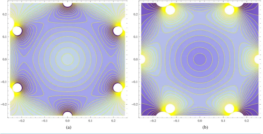
≡EFe −EFh , which demonstrates charge density distribution at the Fermi level µ→0 at low charged carriers concentrations n1 and is shown in Figure 3. S n

( )

takes nonzero values outside of Dirac cone’s corner (non-zero values of the chemical potential µ).

[image:8.595.185.412.478.706.2]

By virtue of turn of the holes valence band (conduction band electrons) at π 6 , the hole liquid is localized so that the electron liquid from its valence band could flow into the vacancies of the hole valence band. Similarly,

(9)

the hole liquid flows into the vacancies of the valence band electrons at some valueµ= ±δ δ, 1. Since the an-nihilation processes are absent, the hole and electron Fermi levels are not at µ=0, and stabilized at some value

=

µ ±δ and, respectively, the Fermi level is dynamic. Therefore, there is a dynamic overlapping of valence and conduction bands, and, respectively, clear graphene turns out to be a metal. The neighborhood with µ→0 is a region where trapped quasiparticles could annihilate; therefore the charged carriers there, are practically absent. This actually is the prohibition for charge carriers to be in the Dirac cone’s corner.

The formed dynamic equilibrium can be disturbed by injection of carriers δn from outside into a forbidden neighborhood µ→0. Then, to restore the balance, the charge carriers will move into the forbidden region with subsequent annihilation e+ →h 2γ and, consequently, having opposite sign free carriers appears in the re-gions of localization. The energy δE of the free carriers is equal to energy of both quanta: δE2ω δγ n. Since δn is small, the “sea” of free quasiparticles is a shallow one. According to Figure 3, due to hyperbolic points, between basins of electrons and holes there are unstable regions, which leads to disintegration of the large “see” into separate small “puddles”. Such “puddles” are experimentally observed at δ_n<₁₀15_m−2

[48].

7. Conclusion

The physical flavors approach N=3 to a quantum field description of graphene electronic properties has been developed. It is based on the Dirac-Hartree-Fock self-consistent field approximation and assumption on antifer-romagnetic ordering of graphene lattice. The approach is a generalization of the known model N=2 of mass-less Dirac fermions in graphene. Its first advantage is that the model N=3 gives symmetric electron and hole band structures, which differ from the band structure model N=2 only by a partial violation of the order of

4

q of the six-fold rotational symmetry of primary Dirac cone and its replicas. In the cone’s corner q →0 the Dirac cone is degenerated. The second advantage is the possibility to account for charged carriers asymmetry stipulated by exchange interaction potential for different sublattices. The third flavor, given by transformations

AB

Σ , ΣBA, gives charged carriers asymmetry and is expressed in dynamical location of the Fermi level and dy-namical localization of electrons and holes.

References

[1] Grushevskaya, G.V., Komarov, L.I. and Gurskii, L.I. (1998) Physics of Solid State, 40, 1802-1805. http://dx.doi.org/10.1134/1.1130660

[2] Gusynin, V.P., Sharapov, S.G. and Carbotte, J.P. (2007) International Journal of Modern Physics B, 21, 4611. http://dx.doi.org/10.1142/S0217979207038022

[3] Peres, N.M.R. (2009) Journal of Physics: Condensed Matter, 21, 323201. http://dx.doi.org/10.1088/0953-8984/21/32/323201

[4] Ziegler, K. (2007) Physical Review B, 75, 233407. http://dx.doi.org/10.1103/PhysRevB.75.233407 [5] Ando, T., Zheng, Y. and Suzuura, H. (2002) Journal of the Physical Society of Japan, 71, 1318-1324.

http://dx.doi.org/10.1143/JPSJ.71.1318

[6] Novoselov, K.S., Geim, A.K., Morozov, S.V., et al. (2004) Science, 306, 666. http://dx.doi.org/10.1143/JPSJ.71.1318 [7] Dean, C.R., Young, A.F. and Meric, I. (2010) Nature Nanotechnology, 5, 722.

http://dx.doi.org/10.1038/nnano.2010.172

[8] Bolotin, K.I., Sikes, K.J., Hone, J., Stormer, H.L. and Kim, P. (2008) Physical Review Letters, 101, 096802. http://dx.doi.org/10.1103/PhysRevLett.101.096802

[9] Du, X., Skachko, I., Barker, A. and Andrei, E.Y. (2008) Nature Nanotechnology, 3, 491-495. http://dx.doi.org/10.1038/nnano.2008.199

[10] Geim, A.K. and Novoselov, K.S. (2007) Nature Materials, 6, 183. http://dx.doi.org/10.1038/nmat1849

[11] Castro, E.V., Ochoa, H., Katsnelson, M.I., Gorbachev, R.V., Elias, D.C., Novoselov, K.S., Geim, A.K. and Guinea, F. (2010) Physical Review Letters, 105, 266601. http://dx.doi.org/10.1103/PhysRevLett.105.266601

[12] Hancock, Y. (2011) Journal of Physics D, 44, 473001. http://dx.doi.org/10.1088/0022-3727/44/47/473001 [13] Kibis, O.V. (2011) Physical Review Letters, 107, 106802. http://dx.doi.org/10.1103/PhysRevLett.107.106802

[14] Elias, D.C., Gorbachev, R.V., Mayorov, A.S., Morozov, S.V., Zhukov, A.A., Blake, P., Ponomarenko, L.A., Grigorie-va, I.V., Novoselov, K.S., Guinea, F. and Geim, A.K. (2012) Nature Physics, 8, 172.

(10)

[15] Rojas-Cuervo, A.M. and Rey-González, R.R. (2013) Asymmetric Dirac Cones in Monatomic Hexagonal Lattices. Ar-Xiv:1304.4576v1 [cond-mat.mes-hall]

[16] Wang, J.R. and Liu, G.Z. (2011) Journal of Physics: Condensed Matter, 23, 155602. http://dx.doi.org/10.1088/0953-8984/23/15/155602

[17] Semenoff, G.W. (1984) Physical Review Letters, 53, 2449. http://dx.doi.org/10.1103/PhysRevLett.53.2449 [18] Wallace, P.R. (1947) Physical Review, 71, 622-634. http://dx.doi.org/10.1103/PhysRev.71.622

[19] Reich, S., Maultzsch, J., Thomsen, C. and Ordejón, P. (2002) Physical Review B, 66, 035412. http://dx.doi.org/10.1103/PhysRevB.66.035412

[20] Novoselov, K.S., Geim, A.K., Morozov, S.V., Jiang, D., Zhang, Y., Katsnelson, M.I., Grigorieva, I.V., Dubonos, S.V. and Firsov, A.A. (2005) Nature, 438, 197-200. http://dx.doi.org/10.1038/nature04233

[21] Fialkovsky, I. and Vassilevich, D.V. (2012) European Physical Journal B, 85, 384. http://dx.doi.org/10.1140/epjb/e2012-30685-9

[22] Falkovsky, L.A. (2011) Low Temperature Physics, 37, 480-484. http://dx.doi.org/10.1063/1.3615524 [23] Falkovsky, L.A. and Varlamov, A.A. (2007) European Physical Journal B, 56, 281-284.

http://dx.doi.org/10.1140/epjb/e2007-00142-3

[24] Falkovsky, L.A. (2008) Physics—Uspekhi, 51, 887-897. http://dx.doi.org/10.1070/PU2008v051n09ABEH006625 [25] Gribov, V.N. (2001) Quantum Electrodynamics. Regular and Chaotic Dynamics Publisher, Izhevsk.

[26] Kaku, M. (1994) Quantum Field Theory: A Modern Introduction. Oxford University Press, Oxford.

[27] Abrikosov, A.A. (1998) Physical Review B, 58, 2788. http://dx.doi.org/10.1103/PhysRevB.58.2788

[28] Katsnelson, M.I. (2006) European Physical Journal B, 51, 157-160. http://dx.doi.org/10.1140/epjb/e2006-00203-1 [29] Kane, C.L. and Mele, E.J. (2005) Physical Review Letters, 95, 226801.

http://dx.doi.org/10.1103/PhysRevLett.95.226801

[30] Huertas-Hernando, D., Guinea, F. and Brataas, A. (2006) Physical Review B, 74, 155426. http://dx.doi.org/10.1103/PhysRevB.74.155426

[31] Min, H., Hill, J.E., Sinitsyn, N.A., Sahu, B.R., Kleinman, L. and MacDonald, A.H. (2006) Physical Review B, 74, 165310. http://dx.doi.org/10.1103/PhysRevB.74.165310

[32] Han, W., McCreary, K., Bao, W., Li, Y., Miao, F., Lau, C.N. and Kawakami, R.K. (2009) Physical Review Letters, 102, 137205. http://dx.doi.org/10.1103/PhysRevLett.102.137205

[33] Han, W., McCreary, K., Pi, K., Wang, W.H., Li, Y., Wen, H., Chen, J.R. and Kawakami, R.K. (2012) Journal of Mag-netism and Magnetic Materials, 324, 369-381. http://dx.doi.org/10.1016/j.jmmm.2011.08.001

[34] Pesin, D. and MacDonald, A.H. (2012) Nature Materials, 11, 409-416. http://dx.doi.org/10.1038/nmat3305

[35] Elias, D.C., Gorbachev, R.V., Mayorov, A.S., Morozov, S.V., Zhukov, A.A., Blake, P., Ponomarenko, L.A., Grigorie-va, I.V., Novoselov, K.S., Guinea, F. and Geim, A.K. (2011) Nature Physics, 7, 701-704.

http://dx.doi.org/10.1038/nphys2049

[36] Ferreira, A., Rappoport, T.G., Cazalilla, M.A. and Neto, A.H.C. (2014) Physical Review Letters, 112, 066601. http://dx.doi.org/10.1103/PhysRevLett.112.066601

[37] Neto, A.H.C., Guinea, F., Peres, N.M., Novoselov, K.S. and Geim, A.K. (2009) Reviews of Modern Physics, 81, 109-162. http://dx.doi.org/10.1103/RevModPhys.81.109

[38] Dirac, P.A.M. (1966) Lectures on Quantum Field Theory. Belfer Graduate School of Science, New York.

[39] Grushevskaya, H.V. and Krylov, G.G. (2013) Int. J. Nonlin. Phen. in Comp. Sys., 16, 189-208.

[40] Rahman, A., Guikema, J.W. and Marković, N. (2013) Asymmetric Scattering of Dirac Electrons and Holes in Gra-phene. arXiv:1304.6318v1 [cond-mat.mes-hall]

[41] Rahman, A., Guikema, J.W. and Marković, N. (2013) Direct Evidence of Angle-Selective Transmission of Dirac Elec-trons in Graphene p-n Junctions. arXiv:1304.5533v1 [cond-mat.mes-hall]

[42] Rossi, E., Bardarson, J.H., Fuhrer, M.S. and Das, S.S. (2012) Physical Review Letters, 109, 096801. http://dx.doi.org/10.1103/PhysRevLett.109.096801

[43] Grushevskaya, H.V. and Krylov, G.G. (2014) Int. J. Nonlin. Phen. in Comp. Sys., 17, 86-96.

[44] Grushevskaya, H.V. and Krylov, G.G. (2013) Electronic Structure and Transport in Graphene: Quasi-Relativistic Dirac- Hartree-Fock Self-Consistent Field Approximation. arXiv:1309.1847 [cond-mat.mes-hall]

(11)

Topology: Effects of Localization. In: Mokshin, A.V., et al., Eds., Dynamical Phenomena in Complex Systems, MOiN RT Publishing, Kazan, 161-180. (in Russian)

[46] Krylova, H. and Hursky, L. (2013) Spin Polarization in Strong-Correlated Nanosystems. LAP LAMBERT Academic Publishing, Saarbrücken.

[47] Messiah, A. (2000) Quantum Mechanics, Vol. 1. Dover Publications, Mineola.