Quantification of Urban Expansion Using Geospatial Technology—A Case Study in Bangalore

http://dx.doi.org/10.4236/ars.2015.44027

Quantification of Urban Expansion Using

Geospatial Technology—A Case Study

in Bangalore

Puspa P. Dash, Ritu Kakkar, V. Shreenivas, P. Jeya Prakash, D. J. Mythri,

K. H. Vinaya Kumar, Vanashree Vipin Singh, R. M. N. Sahai

Centre for Lake Conservation, Environmental Management and Policy Research Institute, Doresanipalya Forest Campus, Bangalore, India

Received 26 October 2015; accepted 20 December 2015; published 23 December 2015

Copyright © 2015 by authors and Scientific Research Publishing Inc.

This work is licensed under the Creative Commons Attribution International License (CC BY). http://creativecommons.org/licenses/by/4.0/

Abstract

Quantification of urban expansion helps us to understand human induced effects on the environ-ment in a temporal scale. Growing urbanization in Bangalore has resulted in demand for more space and resources. Since last 15 years the landuse and landcover of Bangalore area has been changed drastically due to increase in settlement, urban infrastructure, opening of roads and me-tros etc. Using geospatial tools, we studied the changes in landuse and landcover over 19 years (1992-2011) of period and changes in transport network over 41 years (1970-2011) in parts of Bangalore. Thus, the current study shows that the built-up area has been increased drastically, tree cover areas have been converted to agricultural lands and agricultural lands to built-up areas due to urbanization. There are also changes in drainage pattern, transport network and en-croachment of water bodies. Thus the whole environment is getting affected adversely due to un-planned and rapid urban sprawl.

Keywords

Urban Expansion, Land Use, Land Cover, Change Analysis, Satellite Data, GIS

1. Introduction

activi-ties are the main threats to the natural ecosystem. Due to the demand for more space, the LC of the earth has been changing rapidly into several human LU practices such as built-up areas, commercial spaces, transport network etc. The knowledge of LU and LC has become increasingly important as the National plans to over-come the problems of haphazard, uncontrolled development, deteriorating environmental quality, loss of prime agricultural lands, destruction of important wetlands, and loss of fish and wildlife habitat [1].

Both population growth and urbanization are interlinked and continuous phenomenon, so in the present sce-nario there is an urgent need for proper planned development, so that the ecosystem in and around the urban fringes can be saved. The study of LU-LC change analysis has been given more importance after the develop-ment of Remote Sensing (RS) technology since 1980’s. LU study until the late 60’s and early 70’s has been based on conventional surveys which are very expensive and time consuming. The remotely sensed data from space borne sensors provide repetitive coverage and data in digital form which is amenable to computer analysis using GIS [2]. To quantify the amount of changes in land from one form to another, the advanced technology of geospatial analysis (RS and GIS) in temporal domain has given a significant contribution to the world. LU/ LC change has also tremendous effect on water quality, land and air resources, ecosystem processes and function, and climate [3]; biodiversity [4], soil degradation [5] and the ability of natural systems to support life [6]. There are a number of international research projects on dynamics of LU/LC analysis. Some of the examples are The International Geosphere-Biosphere Project (1988) and the LU/LC Change program which were initiated in a bid to construct an updated and accurate database concerning observed changes, their meaning, pace, magnitude and driving forces behind such changes [7]. Quantifying the changes in the landscape is very important for clear un-derstanding of the spatial and structural variability in the LU and their associated ecological effects [8][9].

Pertaining to the growth of Bangalore City, some studies have been done. [10] analysed the changes in land use and land cover pattern using both historical maps and RS imagery. Bangalore urban district LU mapping and LC assessment was carried out jointly by Indian Space Research Organization (ISRO/DOS) and Karnataka State Remote Sensing Agency (1996-2002) as a prototype study for Natural Resources Census (ISRO/KSRSAC, 2005). A comparative assessment has been done by [2] on population, economy, urban sprawl in both Bangalore and Hyderabad cities to analyse the land use changes. Bangalore, which is also known as the city of lakes, gar-den city and pensioner’s paradise, over the period of time, has grown significantly both in technology and ur-banization and has been named as “Silicon Valley”. Bangalore city was awarded “Indira Priyadarshini Vruksha Mitra” by the Central Government in 1980 for its extensive green cover. But today lung space is shrinking in the city and the core areas have lost green cover with increase in concrete structures [11]. The vastly growing popu-lation will turn Bangalore into a “concrete forest” within a time span of 15 - 20 years. This study was conducted to review the past and present situation and trend of urban expansion in part of Bangalore district. The objective of the present study is to analyse the quantity of change of LC into different LU patterns over 19 years period and also changes in transport network and drainage pattern over 41 years of time period by using geospatial technology.

2. Study Area

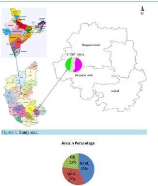
Study area is situated at Latitude 12˚53'53" and Longitude 77˚23'46" of Bangalore district of Karnataka state (Figure 1). The study area consists of 31 villages. The area is chosen in such a manner that, the impact of ur-banization can be studied very clearly. The area is segregated into three different zones on the basis of develop-mental activities. These zones are already developed Sir Mokshagundam Visveswaraiah Layout (SMVL), de-veloping layout Nada Prabhu Kempegowda Layout (NPKL) and yet to develop i.e. Green Belt (GB) area (Figure 2).

3. Materials and Methods

For the current study Arc View 3.2a and Quantum GIS 1.6.0 softwares are used. Toposheets of 1:50,000 scale used to quantify the past roads, drainages, water bodies etc. Landsat data and Aster data were used for landuse (LU)/landcover (LC) classification, current road network, drainage pattern analysis, water bodies and for LU-LC change analysis.

Figure 1. Study area.

NPKL 43% SMVL

34% GB 23%

Area in Percentage

Figure 2. Area covered by different zones in the study area.

digitized and used for further analysis. For changes in land use land cover pattern, Landsat data of 1992, 2000 and Aster data of 2011 were used. On screen visual interpretation method was followed to create the LU/LC maps of 1992, 2000 and 2011. The image elements that are considered for interpretation are tone, texture, size, shape, shadow association and physiography. Google earth data and information collected during the field work are taken for the classification of images into different classes. The interpretation key and field knowledge were utilised for the preparation of LU/LC maps. Intensive field work has been carried out to collect the GPS loca-tions of all the water bodies big to small which are locally named as kere, katte and kunte and also other features and then same was verified on the prepared maps.

To know the gradient of the area, contours are digitized from toposheets and Digital Elevation Model was prepared using Quantum GIS software.

Water spread areas for major water bodies were mapped for two seasons (summer and monsoon) by using GPS tracking method. The water spread area was mapped to know the seasonal reduction in water spread area.

4. Results and Discussion

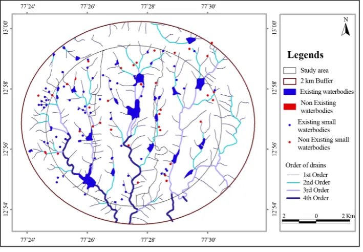
river is flowing in the southern part of the study area. Though these two rivers are flowing outside of the study area, all the drainages are tributaries of Vrishibhavati river. The direction of flow of water is from the north to south as the northern part is having high slope as compared to southern part. The numbering of the streams done by following Strahler stream order (Figure 3) based on a hierarchy of tributaries [12]. The order of drainage in the present area is up to 4th order. 1st and 2nd order drainages are the minor drainages whereas 3rd and 4th order drainages are the major drainages.

4.1. Quantification of Urban Expansion

Bangalore was established during 1537 by Kempe Gowda-I, by building a mud fort. Within the fort, the town was divided into Petesor localities such as Chickpete, Dodpete, Balepete, Cottonpete and other areas earmarked for different trades by artisans [13]. He also built many tanks, temples which have made village Bangalore into a cultural city. After him, his son Kempe Gowda-II has developed the city up to some extent. From 1673-1790 A.D., Mughal Kings Khasim Khan, Hyder Ali, Tipu Sultan ruled the area and built it into a small town of five Kms in circumference. Britishers built many commercial places, railway line etc. Bangalore continued to grow and several public sector industries were set up from 1940-1970 transforming it into a science and technology centre. By 1961, Bangalore had become the 6th largest city in India with a population of 1,207,000. Between 1971 and 1981, Bangalore’s growth rate was 76%, the fastest in Asia. By 1988, the Electronic City had been developed and Bangalore emerged as India’s software capital. Consequently the 1990’s saw a construction boom fuelled by Bangalore’s growing reputation as “India’s Silicon Valley”, which saw many young profes-sionals migrate to the city [13]. This is how the urbanization in Bangalore started and due to all the above said reasons it is expanding day-by-day and there is increasing demand for space. Urban growth is occurring unsci-entifically in the whole area, which is encumbering the natural landscape. Bangalore’s population was three lakhs in 1931 and now the population is more than 80 lakhs (Figure 4).

The above statistics shows the tremendous growth of population in Bangalore city and in order to meet the growing need, the city area is also expanding to the rural fringes.

4.1.1. LU/LC Mapping

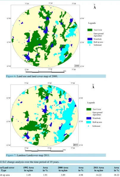
The LU/ LC map has been prepared for 19 years viz, 1992, 2000 and 2011 years respectively. The LU/LC classes derived are: built-up area, open ground/agricultural land, tree cover area and water body. The map of 1992 (Figure 5) indicates that, the tree cover areas are mostly surrounded along the lakes and the drainages. The

1,654,000 2,922,000 4,130,000 5,101,000 8,425,970 174.71 365.65 413.03 492.55 741 0 100 200 300 400 500 600 700 800 0 1,000,000 2,000,000 3,000,000 4,000,000 5,000,000 6,000,000 7,000,000 8,000,000 9,000,000

1971 1981 1991 2001 2011

AR EA POP UL AT ION YEAR Population Area (sq km)

Figure 4. Population statistics of Bangalore over 40 years.

Figure 5. Land use and land cover map of 1992.

tree covers are continuous and less fragments in 1992. While comparing 1992 and 2000 LU/LC maps (Figure 5,

Figure 6), the result indicates that there is increase in built-up areas from 1.49 to 3.89 sq.km (Table 1). In 2011 (Figure 7), map clearly shows that the urbanization has grown extensively in SMVL and covers 18.22% of the area. In the last 19 years, it has been observed that open ground/Agricultural land have been decreased from 53.84 sq.km to 50.26 sq.kms. There is almost 10.8% of the tree cover area has been decreased in past 19 years and at the same time built up area has been increased almost 16.3%. The built up areas which are in small patches have become more prominent and continuous and the tree cover areas are more fragmented.

4.1.2. Transport Network

Figure 6. Land use and land cover map of 2000.

Figure 7. Landuse Landcover map 2011.

Table 1. LU/LC change analysis over the time period of 19 years.

Land use/Land cover Type

1992 Area in sq.km

Area in %

2000 Area in sq.km

Area in %

2011 Area in sq.km

Area in %

Built up area 1.49 1.91 3.89 4.98 14.22 18.22

Open ground/Agriculture 53.84 68.99 52.97 67.88 50.26 64.40

Tree cover 19.52 25.01 18.53 23.74 11.05 14.16

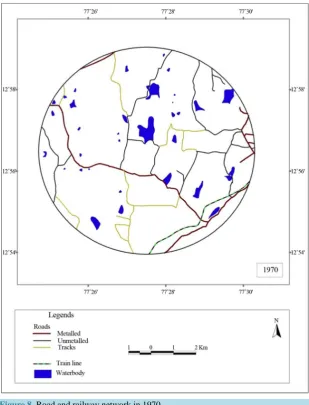
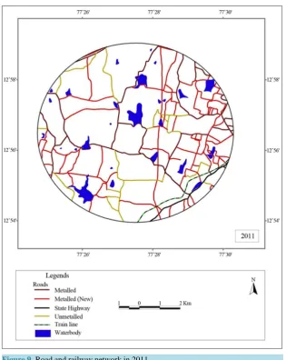
many new unmetalled roads built in the whole study area and one State Highway is passing through the study area. Four water bodies namely, Mangannahalli lake-1 (10%), Manganahalli lake-2 (5%), Ramsandra Chikere (40%) and Komgatta lake (15%) are affected due to the construction of NICE road (Figure 8). As a result, areas of these water bodies have been reduced. Among these fours lakes, Ramsandra Chikere has been affected more. The number of roads has increased in SMV layout due to urbanization and infrastructure development (Figure 8

and Figure 9). There is one railway line present in the Southern part of the study area. This is the only railway line present in the study area and there is no further development in railway line in the last 41 years.

4.1.3. Digital Elevation Modelling (DEM)

Digital Elevation Modelling (DEM) has been created by using geospatial technique to know the gradient of the study area. DEM gives the three dimensional digital representation of a topographic surface. The elevation of the study area varies from 760 m to 900 m. Herohalli village is at the highest peak and Bhimankuppe, Challa-hatta villages are with low terrain in the whole study area. It can be clearly inferred that the gradient of the study area is from the North to South and direction of flow of water is also from the North to South (Figure 10).

4.1.4. Changes in Drainage Pattern

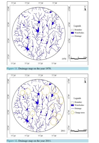
The comparative analysis of drainage pattern of 1970 (Figure 11) and 2011 (Figure 12) gives the inference that few primary drainages from the Northern part of the study area have disappeared. Disappearance of these drain-

Figure 9. Road and railway network in 2011.

Digital Elevation Model

Highest elevation 900 m

Lowest elevation 760 m

Figure 11. Drainage map on the year 1970.

Figure 12. Drainage map on the year 2011.

ages are observed in Herohalli, Gidadakonenahalli, Mallathahalli, Nagdevanahalli and Valgerahalli villages near Kengeri village in the eastern part of the study area. Some changes are also seen in the middle part of Kodige-halli, Sulikere, Kommaghatta villages and in the Western part in Channenahalli and Honniganahatti villages. The change pattern is seen more in the Eastern part due to urbanization. The construction of roads and buildings has affected most of these drainages.

4.1.5. GPS Mapping of Water Spread Area

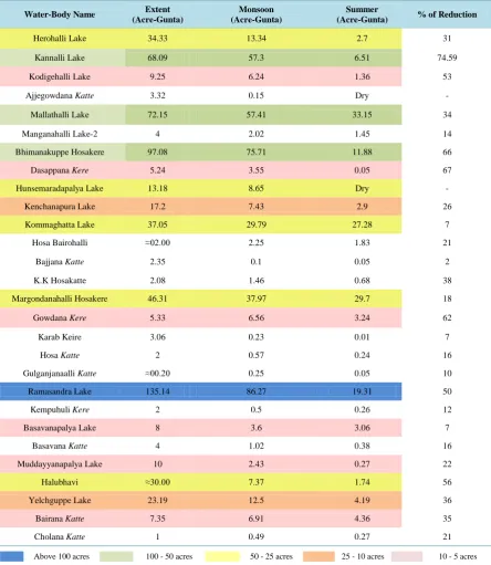
Table 2. GPS water spread area.

Water-Body Name Extent (Acre-Gunta)

Monsoon (Acre-Gunta)

Summer

(Acre-Gunta) % of Reduction

Herohalli Lake 34.33 13.34 2.7 31

Kannalli Lake 68.09 57.3 6.51 74.59

Kodigehalli Lake 9.25 6.24 1.36 53

Ajjegowdana Katte 3.32 0.15 Dry -

Mallathalli Lake 72.15 57.41 33.15 34

Manganahalli Lake-2 4 2.02 1.45 14

Bhimanakuppe Hosakere 97.08 75.71 11.88 66

Dasappana Kere 5.24 3.55 0.05 67

Hunsemaradapalya Lake 13.18 8.65 Dry -

Kenchanapura Lake 17.2 7.43 2.9 26

Kommaghatta Lake 37.05 29.79 27.28 7

Hosa Bairohalli ≈02.00 2.25 1.83 21

Bajjana Katte 2.35 0.1 0.05 2

K.K Hosakatte 2.08 1.46 0.68 38

Margondanahalli Hosakere 46.31 37.97 29.7 18

Gowdana Kere 5.33 6.56 3.24 62

Karab Keire 3.06 0.23 0.01 7

Hosa Katte 2 0.57 0.24 16

Gulganjanaalli Katte ≈00.20 0.25 0.05 10

Ramasandra Lake 135.14 86.27 19.31 50

Kempuhuli Kere 2 0.5 0.26 12

Basavanapalya Lake 8 3.6 3.06 7

Basavana Katte 4 1.02 0.38 16

Muddayyanapalya Lake 10 2.43 0.27 22

Halubhavi ≈30.00 7.37 1.74 56

Yelchguppe Lake 23.19 12.5 4.19 36

Bairana Katte 7.35 6.91 4.36 35

Cholana Katte 1 0.49 0.27 21

Above 100 acres 100 - 50 acres 50 - 25 acres 25 - 10 acres 10 - 5 acres

Ramsandra lake (the biggest lake in the study area which covers 135 acres) has 86.27 acres of water spread area in monsoon season and has reduced to 19.31 acres in summer season (Figure 13). Bhimanakuppe Hosakere, Kannali lake, Margondanahalli Hosakere are the three lakes, which have water spread area in the range of 50 - 100 acres. The actual area of Bhimanakuppe Hosakere is 97.08 acres; the water spread area during monsoon is 75.71 acres and 11.88 acres in summer seasons (Figure 14). Likewise the water spread area for Margondana-halli Hosakere (Figure 15) is 57.41 and 33.15 acres in monsoon and summer season respectively. Table 2

Ramasandra lake

Monsoon

Summer

Figure 13. Seasonal water spread area of Ramasandra lake.

Monsoon

BhimankuppeLake

Summer

Monsoon Season

Summer Season

Margondanahalli lake

Figure 15. Seasonal water spread area of Margondanahalli lake.

5. Conclusion

This study highlighted the urban expansion analysis of Bangalore city by using geospatial technology. The study has analysed the trend of urban growth which is main driver for current land use and land cover changes. Rapid economic devolvement, transformation of city from rural to urban and improvement in standard of living in re-cent decade are the main contributors to the land transformation. From the above study, it is concluded that in SMV layout the entire area is urbanized and few vacant lands are left. The anthropogenic pressure on lakes is higher in the SMVL areas as compared to the others (NPKL and Greenbelt area). The most polluted lake is Bandematta lake in SMVL, which is one of the examples of impact of urbanization on lakes. The city is ex-panding from the East to West. The layout planning for built-up area is demarketed in SMV layout on ground and construction work also in progress in many areas. In NPK layout plans are approved and in another ten years the whole area will be fully urbanized. In the greenbelt area, local houses are there, but not much urbani-zation comes up. In another 10 - 20 years, the green belt area will also be fully urbanized. [11] suggested that the amount of transformation that took place in 30 years is taking place just within 5 years i.e. the acceleration of changes are faster every year. So, the rate of change in ecological spaces and bio-geography of the area is also faster and negative. There are numbers of examples in Bangalore city where the lake lands (Dharmambudhi tank, Karanji tank, Samangi tank, Millers tank, Siddikatte tank, Mathikere tank, Binnypet tank, Juganhalli tank, Chal-laghatta tank, Koramangala tank, etc.) had converted into built-up areas, commercial spaces, as a result of ur-banization. Therefore, before the growth of full urbanization there is an urgent need for proper utilization of land resources with the application of advanced scientific technologies in order to protect the green cover and water bodies along with their drainages present in the urban fringes.

Acknowledgements

special thanks to the former Professor of Fishery, Bangalore University & Former Acting Director, National Assessment and Accreditation Council (NAAC), Dr. S. Ravichandra Reddy for reviewing the project work.

References

[1] Anderson, J.R., Hardy, E.E., Roach, J.T. and Witmer, R.E. (1976) A Land Use and Land Cover Classification System for Use with Remote Sensor Data. Geological Survey Professional Paper 964, United States Government Printing Of-fice, Washington.

[2] Iyer, N.K., Kulkarni, S. and Raghavaswamy, V. (2007) Economy, Population and Urban Sprawl a Comparative Study of Urban Agglomerations of Bangalore and Hyderabad, India Using Remote Sensing and GIS Techniques. PRIPODE workshop on Urban Population, Development and Environment Dynamics in Developing Countries, Nairobi, 11-13 June 2007, 37 p.

[3] Lambin, E.F., Rounsevell, M.D.A. and Geist, H.J. (2000) Are Agricultural Land-Use Models Able to Predict Changes in Land-Use Intensity? Agriculture, Ecosystems & Environment, 82, 321-331.

http://dx.doi.org/10.1016/S0167-8809(00)00235-8

[4] Liu, J. and Ashton, P.S. (1998) FORMOSAIC: An Individual-Based Spatially Explicit Model for Simulating Forest Dynamics in Landscape Mosaics. Ecological Modelling, 106, 177-200.

http://dx.doi.org/10.1016/S0304-3800(97)00191-9

[5] Trimble, S.W. and Crosson, P. (2000) Land Use: U.S. Soil Erosion Rates. Myth and Reality. Science, 289, 248-250. http://dx.doi.org/10.1126/science.289.5477.248

[6] Vitousek, P.M., Mooney, H.A., Lubchenco, J. and Melilo, J.M. (1997) Human Dominated Earth’s Ecosystems. Science,

277, 494-499. http://dx.doi.org/10.1126/science.277.5325.494

[7] Mather, A.S. (1999) Land Use and Cover Change. Land Use Policy, 16, 143.

[8] Turner, M.G. (2005) Landscape Ecology in North America: Past, Present and Future. Ecology, 86, 1967-1974. http://dx.doi.org/10.1890/04-0890

[9] Kabba, V.T.S. and Li, J.F. (2011) Analysis of Land Use and Land Cover Changes, and Their Ecological Implications in Wuhan, China. Journal of Geography and Geology, 3, 104-118.

[10] Behera, G., Nageswara Rao, P.P., Dutt, C.B.S., Manikiam, B., Balakrishnan, P., Krishnamurthy, J., Jagadeesh, K.M., Ganesha Raj, K., Diwakar, P.G., Padmavathy, A.S. and Parvathy, R. (1985) Growth of Bangalore City since 1900 Based on Maps and Satellite Imagery. ISRO Technical Report No.: 55, Trivandrum.

[11] Priya, N. and Hanjagi, A.D. (2009) Land Transformation: A Threat on Bangalore’s Ecology—A Challenge for Sus-tainable Development. Theoretical and Empirical Researches in Urban Management Special Number 1S/April 2009: Urban Issues in Asia.

[12] Horton, R.E. (1945) Erosional Development of Streams and Their Drainage Basins: Hydro-Physical Approach to Quantitative Morphology. Geological Society of America Bulletin, 56, 275-370.

http://dx.doi.org/10.1130/0016-7606(1945)56[275:EDOSAT]2.0.CO;2