Electricity Demand Analysis Using Cointegration and ARIMA Modelling: A case study of Turkey

Munich Personal RePEc Archive

Electricity Demand Analysis Using

Cointegration and ARIMA Modelling: A

case study of Turkey

Erdogdu, Erkan

Energy Market Regulatory Authority, Republic of Turkey

2007

Online at

https://mpra.ub.uni-muenchen.de/19099/

Electricity Demand Analysis Using Cointegration and ARIMA

Modelling: A case study of Turkey

Erkan Erdogdua,b,*

a

Energy Market Regulatory Authority, Ziyabey Cad. No:19 06520 Balgat/ANKARA TURKEY

Abstract

In the early 2000s, the Republic of Turkey has initiated an ambitious reform

program in her electricity market, which requires privatization, liberalization

as well as a radical restructuring. The most controversial reason behind, or

justification for, recent reforms has been the rapid electricity demand growth;

that is to say, the whole reform process has been a part of the endeavors to

avoid so-called “energy crisis”. Using cointegration analysis and ARIMA

modeling, the present article focuses on this issue by both providing an

electricity demand estimation and forecast, and comparing the results with

official projections. The study concludes, first, that consumers’ respond to

price and income changes is quite limited and therefore there is a need for

*

Corresponding author. Tel.: +90-312-2872560 E-mail:erkan@erdogdu.net

URL:http://erkan.erdogdu.net/english

b

economic regulation in Turkish electricity market; and second, that the

current official electricity demand projections highly overestimate the

electricity demand, which may endanger the development of both a coherent

energy policy in general and a healthy electricity market in particular.

Keywords:Turkish electricity demand, cointegration, ARIMA modelling

1. Introduction

The Republic of Turkey (hereafter Turkey) has initiated a major reform

program of her energy market. The reform program entails privatization,

liberalization as well as a radical restructuring of the whole energy sector,

especially electricity industry. Also, an autonomous regulatory body, Energy

Market Regulatory Authority (EMRA), was created to set up and maintain a

financially strong, stable, transparent and competitive energy market.

The most controversial reason behind, or justification for, recent reforms has

been the endeavor to avoid so-called “energy crisis”. Therefore, the present

article focuses on the electricity demand in Turkey by presenting an

electricity demand estimation and forecast. Besides, the econometric

analysis here contributes to extremely limited literature in Turkish energy

studies.

The article is organized as follows. The next section presents a literature

review in energy demand studies. Section three concentrates on the scope of

an overview of data used in the estimation and forecasting process. In

section six, study results are presented; followed by evaluation of these

results in section seven. The last section concludes.

2. Literature Review

The experiences of the 1970s and 1980s led to a blast in the number of

energy demand studies, a trend that has been to some extent revitalized by

the emergence of worries about the emissions of greenhouse gases from the

combustion of fossil fuels. Therefore, since the early 1970s, various studies

of energy demand have been undertaken using various estimation methods1.

In most of these studies the purpose has been to measure the impact of

economic activity and energy prices on energy demand, i.e. estimating

income2 and price3 elasticities, which are of the utmost importance to

forecasting energy demand. The evidence shows long-run income elasticities

about unity, or slightly above, and the price elasticity is typically found to be

rather small (Bentzen and Engsted, 1993).

In most cases, energy demand studies have adopted two different types of

modeling; namely, “reduced form model” and “structural form model”. The

former is a double-log linear demand model under which energy demand is

assumed to be a direct linear function of energy price and real income.

1

Since economic theory and a priori knowledge indicates that the demand for energy in general depends on price and income, most of the studies in this area have been concentrated on these two variables as the major determinants of energy demand.

2

The income elasticity of energy demand is defined as the percentage change in energy demand given a 1% change in income holding all else constant. This measure provides an indication of how demand will change as income changes.

3

Kouris (1981), Drollas (1984) and Stewart (1991) have employed this model

in their studies. Moreover, Dahl and Sterner (1991) report that more than

sixty published studies applied the reduced form model. On the other hand,

the second model is a disaggregated demand model based on the idea that

the demand for energy is derived demand; that is, energy is not demanded

for its own sake rather for the services it provides such as lighting, heating

and power. It separates energy demand into several number of demand

equations and treats it as an indirect, rather than direct, function of energy

price and real income. Pindyck (1979) provides a detailed discussion of the

structural form model. Although structural form model has various

advantages over reduced form model from an economic point of view, its

widespread utilization has been limited by the fact that it requires a large

number of variables compared to the reduced form model.

Another model for energy demand estimation, namely “irreversibility and

price decomposition model”, was first proposed by Wolffram (1971) and

developed by Traill et al. (1978). Originally, it was based on the assumption

that the response to price reductions would be less than that to price

increases. This model was further improved by Dargay (1992) and Gately

(1992), who introduced three-way price decomposition to isolate the effects

on demand of price decrease, price increase below and above the historic

maximum. Some of the work using this method includes that of Dargay and

Gately (1995a, 1995b), Haas and Schipper (1998), Ryan and Plourde (2002),

just to mention a few. However, it is important to note that most of the studies

Despite the relative popularity of the above methods, the long time span

covered by these studies raises serious concerns about the validity of the

fixed coefficients assumption in the electricity demand equation employed by

these methods. This assumption in a double-log functional form of demand

simply implies constant elasticities for the entire sample period under study.

This feature of the model is indeed questionable in light of the changes that

could have taken place in the economy over such a long period of time

affecting the demand for electricity4. Therefore, it is argued that if data is

collected over a relatively long time period to estimate an electricity demand

function, the possibility that the parameters in the regression may not be

constant should be considered. Furthermore; previous methods, in general,

utilize time series data to estimate energy demand but they do not analyze

the data to establish its properties and therefore they implicitly assume the

data to be stationary, meaning that their means and variances do not

systematically vary over time. However, this attractive data feature is lacking

in most cases. Engle and Granger (1987) have developed a technique,

popularly known as “cointegration and error correction method” (ECM), for

analyzing time series properties and estimating elasticities based on this

analysis, which enables full analysis of the properties of the relevant data

before actual estimation. In their study, Engle and Granger have devised a

model estimation procedure and recommended a number of tests, among

which the most notable and commonly used is the Augmented Dickey-Fuller

(ADF) test. Subsequent improvements related to this approach have been in

the form of inclusion of more specific energy-related variables in the model

and the development of new methods to identify cointegrating relationships,

4

amongst which the Autoregressive Distributed Lag Model (ARDL) and the

Johansen Maximum Likelihood Model (JML) – as outlined in Johansen

(1988) – are especially popular.

Since the late 1980s, especially cointegration analysis has become the

standard component of all studies of energy demand; and most scholars

have done their data analysis based on cointegration. The popularity and

widespread use of the cointegration originate from the fact that it justifies the

use of data on non-stationary variables to estimate coefficients as long as the

variables are cointegrated; that is, they have a long-run equilibrium

relationship. Actually, this is also the basic reason for the use of cointegration

technique in this study. The papers written in this area include that of Engle

et al. (1989); Hunt and Manning (1989), Hunt and Lynk (1992), Bentzen and

Engsted (1993, 2001), Fouquet et al. (1993), Hunt and Witt (1995); and

Beenstock and Goldin (1999).

As for the history of energy demand projection in Turkey; although some

efforts for the application of mathematical modeling to simulate the Turkish

energy system were made during the late 1970s, the official use of such

methods in energy planning and national policy making by the Ministry of

Energy and Natural Resources (MENR) was realized only after 1984. The

forecasts made before 1984 were simply based on various best fit curves

developed by the State Planning Organization (SPO) and MENR. The year

1984 has been a milestone for energy planning and estimation of future

MENR use the simulation model MAED5 (Model for Analysis of Energy

Demand) and WASP III (Wicn Automatic System Planning), which were

orig-inally developed by the IAEA (International Atomic Energy Agency) for

determination of the general energy and electricity demands respectively.

Besides, the energy demand model called EFOM-12 C Mark I that was

developed by the Commission of the European Communities in 1984 was

applied to Turkey. Furthermore, Kouris' correlation models were also applied

for forecasting the primary and secondary energy demands in Turkey.

Moreover, the BALANCE and IMPACT models were used in the context of

ENPEP (Energy and Power Evaluation Program) for the long term supply

and demand projections. Finally, State Institute of Statistics (SIS) and SPO

have developed some mathematical models (Ediger and Tatlidil, 2002).

Since 1984, the Ministry (MENR) prepares energy production and demand

projections in accordance with the growth targets given by SPO. Projections

are made taking into account various factors including development,

industrialization, urbanization, technology, conservation and so on. The

figures are revised each year in the light of the performance over the past

year (Ceylan and Ozturk, 2004). Unfortunately, the official forecasts have

consistently predicted much higher values than the consumption actually

occurred.

5

3. Scope of Study

One of the objectives of this article is to estimate a model of electricity

demand in Turkey with a view to obtaining short and long run estimates of

price and income elasticities. Also, an electricity demand forecast constitutes

another aim of the article.

The model to be employed in demand estimation is a dynamic version of

reduced form model, namely “partial adjustment model”. Also, a cointegration

analysis is carried out to analyze the properties of the data. Furthermore, an

annual electricity demand forecast is developed and presented based on

autoregressive integrated moving average (ARIMA) modelling.

4. Theoretical and Methodological Framework

4.1. Cointegration Analysis

4.1.1. Stationarity and Unit Root Problem

Time series data consists of observations, which are considered as

realizations of random variables that can be described by some stochastic

process. The concept of “stationarity” is related with the properties of this

stochastic process. In this paper, the concept of “weak stationary” is adopted;

meaning that the data is assumed to be stationary if the means, variances

and covariances of the series are independent of time, rather than the entire

Nonstationarity can originate from various sources but the most important

one is the presence of so-called “unit roots”. Consider the AR(1) process

below:

t t 1 t

Y  Y_   (1)

where _t denotes a serially uncorrelated white noise error term with a mean

of zero and a constant variance. If  1, equation (1) becomes a random

walk without drift model. If  is in fact 1, we face what is known as the unit

root problem, that is, a situation of nonstationarity. The name ”unit root”6 is

due to the fact that  1. If, however, I I 1  , then the time series Yt is

stationary. The stationarity of time series is so important because correlation

could persist in nonstationary time series even if the sample is very large and

may result in what is called spurious (or nonsense) regression, as showed by

Yule (1926). Granger and Newbold (1974) argue that it is a good rule of

thumb to suspect that the estimated regression is spurious if R2 is greater

than Durbin-Watson d value; that is R2>d.

As easily be concluded from equation (1), the unit root problem can be

solved, or stationarity can be achieved, by differencing and this can be

indicative of the order of integration in the series. The basic idea behind

cointegration is that if a linear combination of nonstationary (1) variables is

stationary; that is (0 ), then the variables are said to be cointegrated. So to

speak, the linear combination cancels out the stochastic trends in the two

(1)

 series and, as a result, the regression would be meaningful; that is, not

6

spurious7. As Granger (1986, p 226) notes, “A test for cointegration can thus

be thought of as a pre-test to avoid ‘spurious regression' situations”.

Therefore, it is vital to specify whether each variable in the model is

stationary or not in order to examine a possible cointegrating relationship

between them. The established way to do so is to apply a formal unit root test

in each series.

4.1.2. The Augmented Dickey-Fuller (ADF) Test

We know that if  1; that is, in the case of unit root, the equation (1)

becomes a random walk model without drift, which we know is a

nonstationary process. The basic idea behind the unit root test of stationary

is to simply regress Yt on its (one-period) lagged value Yt-1 and find out if the

estimated  is statically equal to 1 or not.

For theoretical reasons, equation (1) is manipulated by subtracting Yt-1 from

both sides to obtain:

t t 1 t 1 t

Y Y_   ( 1)Y_   (2)

which can be written as:

t t 1 t Y Y_

     (3)

where    ( 1) and , as usual, is the first difference operator. So, in

practice, instead of estimating equation (2), we estimate equation (3) and test

the null hypothesis that  0. If  0, then  1, meaning that we have a

7

unit root problem and time series under consideration is nonstationary. The

only question is which test to use to find out whether the estimated coefficient

of Yt-1 in equation (3) is zero or not. Unfortunately, under the null hypothesis

that  0 (i.e., 1), the t value of the estimated coefficient of Yt-1 does not

follow t distribution even in large samples; that is, it does not have an

asymptotic normal distribution. Dickey and Fuller (1979) have shown that

under the null hypothesis that  0, the estimated t value of the coefficient of

Yt-1 in equation (3) follows the  (tau) statistic. These authors have also

computed the critical values of the  (tau) statistic. In literature tau statistic or

test is known as the Dickey-Fuller (DF) test, in honor of its discoverers.

In conducting DF test, it is assumed that the error term _t is uncorrelated.

However, in practice the error term in DF test usually shows evidence of

serial correlation. To solve this problem, Dickey and Fuller have developed a

test, known as the augmented Dickey-Fuller (ADF) test. In ADF test, the lags

of the first difference are included in the regression in order to make the error

term _t white noise and, therefore, the regression is presented in the

following form:

m

t t 1 i t i t i 1

Y Y_ Y_



    



To be more specific, we may also include an intercept and a time trend t,

after which our model becomes:

m

t 1 2 t 1 i t i t i 1

Y t Y_ Y_



The DF and ADF tests are similar since they have the same asymptotic

distribution. In literature, although there exist numerous unit root tests, the

most notable and commonly used one is ADF test and, therefore, it is used in

this study.

4.1.3. Cointegration Tests

On the basis of the theory that (1) variables may have a cointegrating

relationship; it is crucial to test for the existence of such a relationship. This

article considers two most commonly used tests of cointegration; namely

Augmented Engle-Granger (AEG) test and cointegrating regression

Durbin-Watson (CRDW) test.

4.1.3.1. Augmented Engle-Granger (AEG) Test

We have warned that the regression of a nonstationary time series on other

nonstationary time series may produce a spurious regression. If we subject

our time series data individually to unit root analysis and find that they are all

(1)

 ; that is, they contain a unit root; there is a possibility that our regression

can still be meaningful (i.e., not spurious) provided that the variables are

cointegrated. In order to find out whether they are cointegrated or not, we

simply carry out our original regression and subject our error term to unit root

analysis. If it is stationary; that is, (0 ), it means that our variables are

cointegrated and have a long-term, or equilibrium, relationship between

stationary, the conventional regression methodology is applicable to data

involving nonstationary time series.

Augmented Engle-Granger test (or, AEG test) is based on the idea described

above. We simply estimate our original regression, obtain the residuals and

carry out the ADF test. In literature, such a regression is called “cointegrating

regression” and the parameters are known as “cointegrating parameters”.

However, since the estimated residuals are based on the estimated

cointegrating parameters, the ADF critical values are not appropriate. Engle

and Granger (1987) have calculated appropriate values and therefore the

ADF test in the present context is known as Augmented Engle-Granger test.

4.1.3.2. Cointegrating Regression Durbin-Watson (CRDW) Test

An alternative method of testing for cointegration is the CRDW test, whose

critical values were first provided by Sargan and Bhargava (1983). In CRDW,

the Durbin-Watson statistic d obtained from the cointegrating regression is

used; but here the null hypothesis8is that d=0, rather than the standard d=2.

The 1 percent critical value to test the hypothesis that the true d=0 is 0.511.

Thus, if the computed d value is smaller than 0.511, we reject the null

hypothesis of cointegration at the 1% level. Otherwise, we fail to reject the

null, meaning that the variables in the model are cointegrated and there is a

long-term, or equilibrium, relationship between the variables.

8

4.2. Partial Adjustment Model

In line with economic theory and a priori knowledge, this study starts with a

single equation demand model expressed in linear logarithmic form linking

the quantity of per capita electricity demand to real energy price and real

income per capita.

The simplest model can be written as:

t 1 t 2 t t

lnE     lnP   ln Y u (6)

where Et is per capita demand for electricity, Pt is the real price of electricity,

Yt is real income per capita, ut is the error term, the subscript t represents

time,  is intercept term; and finally ₁ and ₂ are the estimators of the price

and income elasticities of demand respectively.

This simple “static” model (6) does not make a distinction between short and

long run elasticities. Therefore, instead of this static one, a dynamic version

of reduced form model, called “partial adjustment model”, is used in this

study to capture short-run and long run reactions separately. The partial

adjustment model assumes that electricity demand cannot immediately

respond to the change in electricity price and real income; but gradually

converges toward the long run equilibrium. Suppose that E't is the desired or

equilibrium electricity demand that is not observable directly but given by:

t 1 t 2 t t

and the adjustment to the equilibrium demand level is assumed to be in the

form of

t t 1 t t 1

lnE lnE_  (lnE lnE )_ (8)

where  indicates the speed of adjustment ( 0). Substituting equation (7)

into equation (8) gives:

t t 1 1 t 2 t t t 1

t 1 t 2 t t t 1 t 1

lnE lnE ( lnP ln Y u lnE )

lnE lnP ln Y u lnE lnE

 

 

         

          

t 1 t 2 t t 1 t

lnE     lnP   ln Y   (1 )lnE_  u (9)

where ₁ and ₂ are the short-run price and income elasticities

respectively. The long-run price and income elasticities are given by ₁ and

2

 correspondingly. Since the error term u_t is serially uncorrelated,

consistent estimates of , ₁, ₂ and  can be obtained by OLS (Ordinary

Least Squares).

4.3. Autoregressive Integrated Moving Average Modelling

The publication authored by Box and Jenkins (1978) ushered in a new

generation of forecasting tools, technically known as the ARIMA

methodology9, which emphasizes on analyzing the probabilistic, or

stochastic, properties of economic time series on their own rather than

constructing single or simultaneous equation models. ARIMA models allow

9

each variable to be explained by its own past, or lagged, values and

stochastic error terms.

If we have to difference a time series d times to make it stationary and apply

the ARMA(p,q) model to it, we say the original time series is ARIMA(p,d,q).

The important point to note in ARIMA modelling is that we must have either a

stationary time series or a time series that becomes stationary after one or

more differencing to be able to use it.

ARIMA methodology consists of four steps; namely, identification, estimation,

diagnostic checking and, of course, forecasting. First of all, in the first step,

we need to identify appropriate values of our model; that is, p, d and q. The

chief tools in identification are the autocorrelation function (ACF), the partial

autocorrelation function (PACF), and the resulting correlogram, which is

simply the plots of ACF and PACF against the lag length.

The ACF at lag k, denoted by _k, is defined as

k k

0

  

 (10)

where _k is the covariance at lag k, ₀ is the variance. Since both covariance

and variance are measured in the same units, _k is a unitless, or pure,

number; and lies between -1 and +1.

In time series data the main reason of correlation between Yt and Yt-k

Yt-2, … , Yt-k+1. The partial correlation measures the correlation between

observations that are k time periods apart after controlling for correlations at

intermediate lags; that is, it removes the influence of these intervening

variables. In other words, partial autocorrelation is the correlation between Yt

and Yt-k after removing the effect of intermediate Y’s.

If we find out, as a result of visual inspection of correlogram and/or formal

unit root tests, that our data is nonstationary; we need to make it stationary

by differencing until nonstationary fades away. Then, based on the stationary

data after differencing and its correlogram, we identify the appropriate values

of our model; that is, p, d and q.

In the second step; that is, estimation, the model based on the results from

the first step is constructed and estimated, which is followed by diagnostic

checking in the third step. To check whether the model is a reasonable fit to

the data or not, we collect residuals from the estimation in previous step and

check whether any of the autocorrelations and partial correlations of the

residuals is individually statistically significant or not. If they are not

statistically significant, then it means that the residuals are purely random

and there is no need to look for another ARIMA model. In the final step,

forecasting is carried out based on the constructed and checked ARIMA

5. Overview of Data

The data used in the estimation process is quarterly time series data on real

electricity prices, real GDP per capita and net electricity consumption per

capita for the period 1984-2004, a total of 84 observations. The data is

obtained from the “International Energy Agency” (IEA), the “Organisation for

Economic Co-operation and Development” (OECD), the “International

Monetary Fund” (IMF) and some national institutions of Turkey; namely, the

“State Institute of Statistics” (SIS), the “Turkish Electricity Transmission

Company” (TEIAS), Undersecretariat of Treasury and State Planning

Organization (SPO).

Since the data on net electricity consumption, population and GDP is not

available quarterly, the annual series on these data are converted into

quarterly data by linear interpolation so as to make use of them together with

quarterly data on electricity prices. Specification of data and their sources are

summarized in Appendix A.

Since one of the main aims of this study is to get elasticities of electricity

demand, the series were transformed into natural logarithms so that direct

estimates of elasticities can be obtained10. Graphs below show time series

plots of natural logarithms of real electricity prices (LP), real GDP per capita

(LY) and real net electricity consumption per capita (LE).

10

[ “image1.bmp” goes here ]

Figure 1.Time Series Plots of Natural Logarithms of LP, LY and LE

A close look at the graphs reveals that there are trends in the variables with

the exception of LP, which fluctuates within an interval. Visual inspection of

the plotted data also indicates that LY and LE have non-constant means and

non-constant variances; that is, they seem to be non-stationary.

6. Presentation of Study Results

6.1. Partial Adjustment Model

Using quarterly data discussed in the previous section, the reduced form

model is estimated11. Equation (6) is estimated as follows:

t t t

lnE  5.12 1.17 lnP 1.18 ln Y (11)

In this model, p-values of , ₁ and ₂ are all within acceptable range and

the null hypothesis that one of these coefficients is zero can be rejected at

the 2% significance level. As for “goodness-of-fit” measures, “R-squared” and

“Adjusted R-squared” values are about 0.38 and 0.36 respectively; which

cannot be regarded as high enough for an appropriate model.

11

As to serial correlation, Durbin-Watson statistic in our estimation output is

very close to 0.14, indicating the existence of serial correlation in the

residuals. The p-value of the F-statistics is almost zero; so we can reject the

null hypothesis that all slope coefficients in the regression are zero.

Although the coefficients of price and income have correct signs12,

econometric indicators imply that this equation may be misspecified.

Therefore, the lagged dependent variable, lnEt-1, is added in the

right-hand-side of the equation (6) so as to obtain partial adjustment model in equation

(9), estimation of which gives the following result.

t t t t 1

lnE  0.04 0.01lnP 0.01ln Y 0.99 lnE_ (12)

This new model is clearly better than the first one. First of all, the coefficients

of price and income have still correct signs. Second, p-values of all

coefficients, with the exception of intercept term, are within acceptable range

and they are significant at 2% significance level13. Third, “R-squared” and

“Adjusted R-squared” measures in this model are about 1, meaning that the

regression fits almost perfectly. Finally, p-value of the F-statistics is still zero.

Based on this model, the estimated short-run and long-run elasticities of

demand are as follows14:

12

The economic theory states that there is an inverse relationship between demand and price; and a positive relation exists between demand and income.

13

However, the p-value of the intercept term (0.44) is so high that we cannot reject the zero null hypotheses even at the 40% significance level!

14

Relying on the notation in equation (9), estimated parameters are as follows:   0.041010   1 0.012257  2 0.014779 (1  ) 0.986500

Table 1.Elasticities of Demand for Electricity in Turkey, based on Conventional Partial Adjustment Model

Short-run Long-run

Price Elasticity -0.0123 -0.9079

Income Elasticity 0.0148 1.0947

There seems to be a substantial difference between short-run and long-run

elasticities of demand because, in this model, the speed of adjustment to the

long-run equilibrium demand level is so close to 0 ( 0.0135). The other,

and probably more striking, outcome from this model is the fact that although

short-run elasticities are extremely low, less than 0.02; the long-run response

to both price and income changes is exceptionally high. For instance,

according to this model, if real income doubles (or, increases by 100%) in

Turkey, the demand for electricity increases by 109% in the long run.

Similarly, if real price of electricity declines by 100%, the demand increases

by 91% in the long run.

There is, however, a possibility that the OLS results may be misleading due

to inappropriate standard errors because of the presence of

heteroskedasticity. In order to test whether error terms are heteroskedastic or

not, White heteroskedasticity test (without cross terms) is carried out. The

probability value of 0.146 in this test indicates that they are not jointly

significant even at 10% significance level; meaning that error terms are not

heteroskedastic in our model.

We need also to test for serial correlation. Breusch-Godfrey Serial

test strongly indicates the presence of serial correlation in the residuals. In

the presence of serial correlation, the OLS estimators are still unbiased as

well as consistent and asymptotically normally distributed, but they are no

longer efficient, meaning that standard errors are estimated in the wrong way

and, therefore, usual confidence intervals and hypotheses tests are

unreliable. Moreover, usually, the finding of autocorrelation is also an

indication that the model is misspecified. Newey and West (1987) proposed a

general covariance estimator that is consistent in the presence of both

heteroskedasticity and autocorrelation. Thanks to Newey-West procedure15,

we can still use OLS but correct the standard errors for autocorrelation.

However, when we correct the standard errors for autocorrelation, p-values

of all coefficients become insignificant even at 10% significance level,

supporting the previous indication that the model is misspecified.

Since it is obvious that conventional partial adjustment model is not the

appropriate one in our case; after experimenting with various functional

forms, the model below is specified and estimated.

t 0 1 t 2 t 3 t 2 4 5 t 2 t

lnE     lnP   ln Y   lnP_    t lnE_   (13)

where lnEt-2 and lnPt-2 are the second lag of natural logarithms of demand

and real price respectively; and t is a trend that increases by one for each

observation16.

15

It is important to point out that the Newey-West procedure is strictly speaking valid in large samples and may not be appropriate in small ones. Since we have 84 observations, our sample may be regarded as reasonably large.

16

This last model is obviously the best one. The coefficients of price and

income have correct signs. P-values of all coefficients, without exception, are

significant at 5% significance level. “R-squared” and “Adjusted R-squared”

measures indicate that the regression fits almost perfectly. P-value of the

F-statistics is zero. White heteroskedasticity test (without cross terms) and

Breusch-Godfrey Serial Correlation LM Test are carried out once more for

the new model and the results indicate that we have no heteroskedasticity in

our model but there exists serial correlation in the residuals. In order to

correct the standard errors for autocorrelation, the model is re-estimated by

OLS with Newey-West procedure and it is seen that all coefficients are still

significant at 5% significance level.

Although all econometric indicators support the appropriateness of this

model, a formal test for functional form, namely Ramsey’s RESET test, is

also carried out to make sure that our specification is correct. This test does

not indicate a specification problem in our model at the 5% level of

significance. That is, the model appears to be free from misspecification.

Based on these results, it seems that we need to respecify reduced form

model for Turkish case. First of all, we need to readjust the desired or

equilibrium electricity demand level (E't) in partial adjustment model as

follows:

t 1 t 2 t 3 t 2 4 t

lnE     lnP   ln Y   lnP_   t u (14)

Second, based on the model represented by equation (13), it is clear that

partial adjustment process in Turkey operates as follows:

t t 2 t t 2

lnE lnE_  (lnE lnE_ ) (15)

Substituting equation (14) into equation (15) and rearranging gives:

t 1 t 2 t 3 t 2 4 t 2 t

lnE     lnP   ln Y   lnP_     t (1 )lnE_  u (16)

In order to simplify notation, equation (16) can be rewritten as:

t 0 1 t 2 t 3 t 2 4 5 t 2 t

lnE     lnP   ln Y   lnP_    t lnE_   (17)

where   ₀ ,   _{1 1},   _{2 2},   _{3 3},   _{4 4},    ₅ (1 ) and

t ut

   . In equation (17)17, ₁ and ₂ are the short-run price and income

elasticities respectively. The long-run price and income elasticities are given

by ₁ and ₂ correspondingly. Therefore, based on our estimation results

given below, the short-run and long-run elasticities of demand for electricity in

Turkey are as follows18:

lnE_t 0.653-0.041lnP_t 0.057ln Y_t 0.017lnP_{t 2} 0.002t0.862lnE_{t 2} (18)

17

Please note that equations (17) and (13) are identical.

18

Relying on the notation in equation (17), elasticities are obtained as follows:   1 1-0.041   2 2 0.057 (1  ) 0.862

Table 2. Elasticities of Demand for Electricity in Turkey, based on Readjusted Partial Adjustment Model

Short-run Long-run

Price Elasticity -0.041 -0.297

Income Elasticity 0.057 0.414

Now, there seems to be less difference between short-run and long-run

elasticities of demand because, in this new model, the speed of adjustment

to the long-run equilibrium demand level ( 0.138) is much higher, meaning

that now it takes demand less time to reach long run equilibrium.

Furthermore, it is clear that the long run demand is relatively elastic

compared to short run demand. Moreover, the level of income has more

effect on demand than that of prices. As also suggested by economic theory,

the demand is most responsive to income changes in the long run. According

to this model, in Turkey, if real income increases by 100%, electricity demand

increases by 41% in the long-run.

6.2. Cointegration Analysis

As indicated before, since it is critical to find out whether the results obtained

from our model are meaningful (i.e., not spurious) or not, let me apply formal

unit root tests in each series to test the reliability of our estimates.

6.2.1. The Augmented Dickey-Fuller (ADF) Test

The established standard procedure for cointegration analysis is to start with

Dickey-Fuller (ADF) test is used to test for the presence of unit roots and

establish the order of integration of the variables in the model. The table

below shows the results of the unit root tests19 from estimation of equation

(5). The null hypothesis of the test is that there is a unit root against the

alternative one that there is no unit root in the variables.

Table 3. Summary of ADF Tests for Unit Roots in the Variables (in level form with a trend and intercept)

Variable ADF Test Statistic Results

LNE -1.008983 Fail to reject the null

LNP -2.627504 Fail to reject the null

LNY -2.614160 Fail to reject the null

Note:The ADF statistic at 5% significance is -3.466248.

The ADF statistics for the natural logarithms of electricity demand (LNE), real

electricity prices (LNP) and real income (LNY) are all insignificant at 5

percent level of significance, which leads to non-rejection of the null

hypothesis that there is a unit root problem in the variables. Based on ADF

test, it is obvious that the variables are non-stationary.

As mentioned previously, differencing has the effect of making the variables

stationary. The table below summarizes the results of unit root tests for the

differenced variables.

19

Table 4.Summary of ADF Tests for Unit Roots in the Variables (in 1st difference form with a trend and intercept)

Variable ADF Test Statistic Results

LNE -4.569026 Reject the null

LNP -13.98314 Reject the null

LNY -38.88917 Reject the null

Note:The ADF statistic at 5% significance is -3.466966.

The ADF statistics for the first difference variables are all significant at 5

percent level of significance, which leads to rejection of the null hypothesis

that there is a unit root problem in the variables. Based on ADF test, it is

apparent that the first difference variables are stationary, which implies that

the variables are integrated of order one, (1).

6.2.2. Cointegration Tests

6.2.2.1. Augmented Engle-Granger (AEG) Test

The residuals from the estimation of equation (17) were used to test for the

existence of cointegrating relationship between the variables. The null

hypothesis is that the residuals have a unit root problem against the

alternative that the variables cointegrate. The result of AEG test20 is

presented in the table below.

20

Table 5.Summary of AEG Test Output for Equation (17)

Variable ADF Test Statistic Result

Residuals -5.3643 Reject the null

Note:95% critical value for the Dickey-Fuller statistic is -4.9387.

It is clear that absolute value of ADF test statistic is more than the critical

value, meaning that the null hypothesis is rejected. To reject the null

hypothesis implies that the residuals have not a unit root problem; i.e., they

are stationary. It can therefore be concluded that, based on the AEG method,

the variables are cointegrated.

6.2.2.2. Cointegrating Regression Durbin-Watson Test

Since cointegration is very crucial to the reliability of estimated parameters, a

second test, namely CRDW test, was carried out to make sure that the

variables in this study are definitely cointegrated. The Durbin-Watson statistic

for the regression represented by equation (17) is 0.559, which is above the

1% critical value of 0.511. Therefore, we fail to reject the null hypothesis of

cointegration at the 1% level, which reinforces the finding on the basis of the

AEG test.

To sum up, our conclusion based on both the AEG and CRDW tests is that

the variables LNE, LNP and LNY are cointegrated. Although they individually

exhibit random walks, there seems to be a stable long-run relationship

Based on these results, we may conclude that the appropriate model for

Turkish electricity demand is the one represented in equation (17) and that

our estimates are reliable; that is, not spurious.

6.3. Electricity Demand Forecast for Turkey: 2005-2014

6.3.1. Data and Methodology

Before starting the forecast, it is important to make some points clear. First of

all, data used here is annual data covering the period 192321-2004, a total of

82 observations. Also, unlike previous section, the data here is not converted

into natural logarithms and, therefore, the unit is GWh.

In literature, there are five main approaches to economic forecasting based

on time series data; namely, (1) exponential smoothing methods, (2)

single-equation regression models, (3) simultaneous-single-equation regression models,

(4) autoregressive integrated moving average models (ARIMA), and (5)

vector autoregression. Although still used in some areas, the first group of

models is now supplanted by the other four methods; therefore, we don’t use

them in this study. Taking into account rather low estimates of elasticities

obtained in previous section22, it seems better not to include price and

income variables in the forecasting process and “let the demand data speak

for itself”, which is the main philosophy behind ARIMA modelling. Since the

second, third and the fifth group of models require the inclusion of price,

21

The Republic of Turkey was founded in 1923.

22

income and some other variables in the forecasting process; they are also

not used here. In short, this section develops an electricity demand forecast

for Turkey based on ARIMA modelling.

6.3.2. Development of the Model

As mentioned before, ARIMA modelling consists of four steps. In the first

step, namely identification step, we need to identify the appropriate

parameters in our model, that is, ARIMA(p,d,q). The figure below provides us

with the correlogram up to 40 lags, or the plots of ACF and PACF against the

lag length of 40.

[ “image2.bmp” goes here ]

Figure 2.The Correlogram of Turkish Electricity

Consumption Data up to 40 lags

The column labeled AC and PAC are the sample autocorrelation function and

the sample partial autocorrelation function respectively. Also the diagrams of

AC and PAC are provided on the left. The solid and dashed vertical lines in

the diagram represent the zero axis and 95% confidence interval

respectively. From this figure, two facts stand out: First, the autocorrelation

coefficient starts at a very high value at lag 1 (0.937) and declines very

slowly; and ACF up to 16 lags are individually statistically significant different

from zero as they are all outside the 95% confidence bounds. Second, after

statistically insignificant. These two facts strongly support the idea that the

electricity consumption time series is nonstationary. It may be nonstationary

in mean or variance, or both.

Since the data is nonstationary, we have to make it stationary. The figures

below show the correlograms of the first and second differenced data up to

40 lags.

[ “image3.bmp” goes here ]

Figure 3. The Correlogram of the First-Differenced Data up to 40 lags

[ “image4.bmp” goes here ]

Figure 4. The Correlogram of the Second-Differenced Data up to 40 lags

We still observe a trend in the first-differenced consumption time series but

this trend disappears in the second-differenced one, perhaps suggesting that

the second-differenced data is stationary. A formal application of the ADF

unit root test shows that that is indeed the case.

In Figure 4, we have a much different pattern of ACF and PACF. The ACFs

at lags 1, 3 and 4; and PACFs at 1, 2, 4, 6 and 13 seem statistically different

from zero. But at all other lags, they are not statistically different from zero. If

identified this as an AR(1) model. Let us therefore assume that the process

that generated the second-differenced consumption is at most an AR(13)

process. Since from the partial correlogram we know that only the AR terms

at lag 1, 2, 4, 6 and 13 are significant, we only need to include these AR

terms in our model. Therefore at the end of the first step we may conclude

that the original time series is ARIMA(13,2,0); that is, the second differenced

stationary data can be modeled as an ARMA(13,0) process.

The second step in ARIMA modelling is estimation. Let * t

E denote the

second-differenced data. Then, in line with the conclusion in the first step, our

model is:

    

            

* * * * * *

t 1 t 1 2 t 2 4 t 4 6 t 6 13 t 13 t

E E E E E E u (19)

Using EViews, we obtained the following estimates:

* * * * * *

t t 1 t 2 t 4 t 6 t 13

E 275.93 0.56E _ 0.44E_ 0.62E_ 0.56E_ 0.54E_ (20)

In the third step; that is, diagnostic checking, we obtain residuals from (20)

and get the ACF and PACF of these residuals up to lag 40 in order to check

that the model represented by equation (20) is a reasonable fit to the data.

The estimated ACF and PACF are shown below.

[ “image5.bmp” goes here ]

As can be seen in Figure 5, none of the autocorrelations and partial

correlations is individually statistically significant. In other words, the

correlograms of both autocorrelation and partial autocorrelation give the

impression that the residuals estimated from regression (20) are purely

random. Hence, there is not any need to look for another ARIMA model.

The final step is forecasting. However, we need to integrate the

second-differenced series to obtain the forecast of consumption rather than its

changes. We know that the following formula integrates data from

second-differenced form into level form.

 

  

*

t t t 1 t 2

E E 2E E (21)

If we transform all variables in equation (19) based on this formula and

rearrange it, our model becomes:

Et =  (2 ₁)E_{t 1}     ( ₂ 2 ₁ 1)E_{t 2}    ( ₁ 2 ₂)E_{t 3}

   

   ( _{2 4})E_{t 4} 2 ₄E_{t 5}   ( _{4 6})E_{t 6} 2 ₆E_{t 7} (22)

   

₆E_{t 8} ₁₃E_{t 13}  2 ₁₃E_{t 14} ₁₃E_{t 15}u_t

The values of , ₁, ₂, ₄, ₆ and ₁₃ are already known from the

estimated regression (20) and ut is assumed to be zero, which enables us to

convert equation (22) into equation (23). Using equation (23), we may easily

obtain the forecast values for the period 2005-2014.

Et = 275.93 1.44E _{t 1} 0.32E_{t 2} 0.32E_{t 3} 1.06E_{t 4}

   

1.23E_{t 5}1.17E_{t 6}1.11E_{t 7}0.56E_{t 8} (23)

  

6.3.3. Validation

Before presenting the results, it is useful to validate the present model with

observed data. In order to do this, electricity demand is calculated by

equation (23) supposing that present year is 1999; that is, five years

observed data is used for validation. As can be seen in the table below, the

results from ARIMA model deviates from the observed data 2.2% on

average, which may definitely be regarded as within the acceptable range.

Table 6. Validation of ARIMA Modelling

Year Forecasted Net Electricity Consumption (GWh) Annual % Change Index (1999=100) Actual Net Electricity Consumption (GWh) Annual % Change Index (1999=100) Absolute Value of Deviation

Deviation as a Percentage of

Actual Consumption

2000 98,788 8.3 108 98,296 7.8 108 492 0.5

2001 101,167 2.4 111 97,070 -1.2 106 4,097 4.2

2002 105,143 3.9 115 102,948 6.1 113 2,195 2.1

2003 111,053 5.6 122 111,766 8.6 123 713 0.6

2004 112,466 1.3 123 116,561 4.3 128 4,095 3.5

Note: Average deviation as a % of actual consumption is 2.2

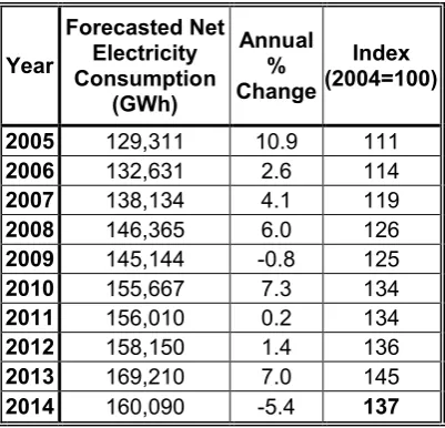
6.3.4. Presentation of the Results

By using equation (23), net electricity demand forecasts are obtained for

Turkey up to the year 2014. As given below, the results from ARIMA

modelling clearly indicate that average annual percentage increase in

Table 7. Demand Forecast for Turkey, 2005-2014

Year

Forecasted Net Electricity Consumption

(GWh)

Annual % Change

Index (2004=100)

2005 129,311 10.9 111

2006 132,631 2.6 114

2007 138,134 4.1 119

2008 146,365 6.0 126

2009 145,144 -0.8 125

2010 155,667 7.3 134

2011 156,010 0.2 134

2012 158,150 1.4 136

2013 169,210 7.0 145

2014 160,090 -5.4 137

Note: Average annual % change is 3.3

7. Evaluation of Study Results

As a result of estimation and forecasting procedure outlined above, the

results given in Table 2 and Table 7 are obtained. Having obtained both the

elasticities of electricity demand in Turkey and forecasted values for this

demand, let me interpret the results and compare them with the official

estimates that are available from TEIAS (2005c).

The estimated elasticities indicate that the price and income elasticities of

electricity demand in Turkey are quite low, meaning that there is definitely a

need for economic regulation in Turkish electricity market. Otherwise, since

consumers do not react much especially to price increases, the firms with

monopoly power (or those in oligopolistic market structure) may abuse their

As to forecasted net electricity consumption values, it is obvious that there

exists an electricity demand growth in Turkey; and in the following decade

(i.e., 2005-2014), based on ARIMA modelling, we may argue that the

demand will continue to increase at an annual average rate of 3.3% and will

turn out to be 160,090 GWh in 2014, corresponding to a 37% increase

compared to 2004 demand level.

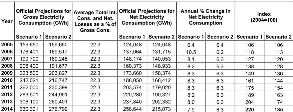
As for comparison of our results with official demand projections, the official

projections are available from TEIAS (2005c) and provided below. However,

the official forecasts are for gross demand; and, therefore, they need to be

converted into net consumption for a meaningful comparison. The details of

this conversion are provided in Appendix B and the result is presented in the

table below. Also, official estimates are based on two different scenarios and

therefore formulated in two different ways. Average annual percentage

increase in net electricity consumption is 8.2% in Scenario 1; and 6.3% in

Scenario 2.

Table 8. Official Projections for Electricity Demand

Year

Official Projections for Gross Electricity Consumption (GWh)

Average Total Int. Cons. and Net. Losses as a % of

Gross Cons.

Official Projections for Net Electricity Consumption (GWh)

Annual % Change in Net Electricity Consumption

Index (2004=100)

Scenario 1 Scenario 2 Scenario 1 Scenario 2 Scenario 1 Scenario 2 Scenario 1 Scenario 2

2005 159,650 159,650 22.3 124,048 124,048 6.4 6.4 106 106

2006 176,401 169,517 22.3 137,064 131,715 10.5 6.2 118 113

2007 190,700 180,248 22.3 148,174 140,053 8.1 6.3 127 120

2008 206,400 191,677 22.3 160,373 148,933 8.2 6.3 138 128

2009 223,500 203,827 22.3 173,660 158,374 8.3 6.3 149 136

2010 242,021 216,747 22.3 188,050 168,412 8.3 6.3 161 144

2011 262,000 230,399 22.3 203,574 179,020 8.3 6.3 175 154

2012 283,501 244,951 22.3 220,280 190,327 8.2 6.3 189 163

2013 306,100 260,401 22.3 237,840 202,332 8.0 6.3 204 174

2014 330,301 276,799 22.3 256,644 215,073 7.9 6.3 220 185

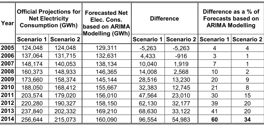
The table below compares the results from ARIMA modelling with official

projections based on two different scenarios.

Table 9. The Comparison of ARIMA Results with Official Projections

Year

Official Projections for Net Electricity Consumption (GWh)

Forecasted Net Elec. Cons. based on ARIMA Modelling (GWh)

Difference

Difference as a % of Forecasts based on

ARIMA Modelling

Scenario 1 Scenario 2 Scenario 1 Scenario 2 Scenario 1 Scenario 2

2005 124,048 124,048 129,311 -5,263 -5,263 4 4

2006 137,064 131,715 132,631 4,433 -916 3 1

2007 148,174 140,053 138,134 10,040 1,919 7 1

2008 160,373 148,933 146,365 14,008 2,568 10 2

2009 173,660 158,374 145,144 28,516 13,230 20 9

2010 188,050 168,412 155,667 32,383 12,745 21 8

2011 203,574 179,020 156,010 47,564 23,010 30 15

2012 220,280 190,327 158,150 62,130 32,177 39 20

2013 237,840 202,332 169,210 68,630 33,122 41 20

2014 256,644 215,073 160,090 96,554 54,983 60 34

The most outstanding outcome from the comparison is the fact that there is a

substantial difference between official projections and forecasts based on

ARIMA modelling. If we suppose that ARIMA results are valid; for 2014,

Scenario 1 and 2 inflate electricity demand by 60% and 34% respectively. To

put it in a different way, if we take electricity demand in 2004 as 100 units;

ARIMA modelling suggests that the demand will turn out to be 137 units in

2014, while official projections imply that it will turn out to be either 220 or

185 units depending on the scenario adopted.

There exist two important points to keep in mind while evaluating (and

perhaps using) these results. First of all, forecasting, especially in energy

variations are to be expected depending on the model’s underlying

assumption(s). Like all other models, ARIMA modelling is based on some

assumption(s) and, of course, there is a direct link between the accuracy of

the forecast and the validity of the underlying assumption(s). The main

assumption behind ARIMA modelling is that the already existing trends in

electricity consumption will more or less repeat themselves in the future.

Despite the fact that this is a widely used, essential and reasonable

assumption; some unanticipated events may also occur and it is always very

difficult, if not impossible, to foresee such "unexpected" events that have a

potential to completely change the electricity demand trend in Turkey

reducing the precision of the forecasts presented here. Second, due to

nature of ARIMA modelling and the low elasticities obtained, present study

has only employed net total consumption data for forecasting. There is an

apparent need for further work with more variables that will examine the

demand of different sectors (e.g., industry, households etc.) separately,

which is not only essential for policy formulation in Turkey but also will make

more detailed and accurate understanding of the trends possible.

Ozturk et al. (2005) conclude that official total electricity demand projection

for the period of 1996–2001 overestimated demand by 36% either due to

inappropriateness of the model used or in order to justify the construction of

new electric power plants to use excess amount of natural gas. In line with

this conclusion; in this study, we find that the official net electricity

consumption projection for 2014 again overestimates demand at least by

8. Conclusion

The main objectives of this article have been, first, to estimate short and long

run price and income elasticities of electricity demand in Turkey; and,

second, to forecast future growth in this demand using ARIMA modelling and

compare the results with official projections.

In the course of study, elasticities are obtained and it is found out that they

are quite low, implying that consumers’ respond to price and income changes

is quite limited; and, therefore, there is a need for economic regulation in

Turkish electricity market. Then, an ARIMA model is developed and used to

forecast future net electricity consumption in Turkey. Based on forecasts

obtained, it is clear that the current official projections highly overestimate the

electricity demand in Turkey.

Developing countries like Turkey should plan very carefully about their

energy demand for critical periods, such as economic crises that frequently

hit them. For instance, economic crisis hit Turkey three times in the last

decade, once in 1994 and the others in 2000 and 2001. During these

periods, energy consumption shows fluctuations and presents a decreasing

trend. After the economic crises, the energy consumption recovers and

shows about the same trend as before the economic crises. Therefore,

official energy projections should be formulated in such a way that possible

crises are taken into account. Moreover, all related bodies in Turkey should

take necessary steps to find out the reasons for apparently misleading

projections. In this context; the market regulator, EMRA, is especially

responsible for development of healthy forecasts, which is one of the most

important determinants in the success of recent energy market reforms in

Turkey. Future energy consumption in Turkey have consistently been

predicted much higher values than actually occurred. It should be kept in

mind that it is almost impossible to create a well-functioning electricity market

under these conditions. In addition; while developing forecasts, the emphasis

should be on the development and use of appropriate data and econometric

techniques which are open to debate, rather than some computer packages

for demand estimation provided by various international organizations or,

even worse, the methods in which the demand is determined as a result of a

bargaining process among various public bodies.

It is believed that the elasticities, forecasts and the comments presented in

this paper would be helpful to policy makers in Turkey for future energy policy

Acknowledgements

I would like to thank my supervisor, Joanne Evans (Lecturer in Economics, University of Surrey, UK), for all her helpful comments and continuous encouragement during the writing of the dissertation on which this paper is constructed. I would also like to thank Lester C. Hunt (Professor of Energy Economics, University of Surrey, UK); Paul Appleby (BP plc, UK); Gürcan Gülen (Senior Energy Economist, University of Texas, USA) and David Hawdon (Senior Lecturer in Economics, University of Surrey, UK) for priceless comments on the final draft. I am also grateful to the British Government through the Foreign and Commonwealth Office for awarding me the British Chevening Scholarship that financed my studies in the UK. I also extend my thanks to the British Council for excellent administration of the scholarship. Besides, I am indebted to the Turkish Government through the Energy Market Regulatory Authority both for granting me a study leave to undertake my academic work in the UK and for the financial support towards my studies there.

I would also like to thank anonymous referees for their very helpful comments on an earlier draft of the paper. The author is, of course, responsible for all errors and omissions.

References

Beenstock, M., Goldin, E., 1999. The demand for electricity in Israel. Energy Economics, 21:2, 168-183.

Bentzen, J., Engsted, T., 1993. Short- and long-run elasticities in energy demand: A cointegration approach. Energy Economics, 15:1, 9-16.

Bentzen, J., Engsted, T., 2001. A revival of the autoregressive distributed lag model in estimating energy demand relationships. Energy, 26:1, 45-55.

Box, G.P.E., Jenkins, G.M., 1978. Time Series Analysis: Forecasting and Control, Holden Day: San Francisco.

Ceylan, H., Ozturk, H.K., 2004. Estimating Energy Demand of Turkey based on Economic Indicators Using Genetic Algorithm Approach. Energy

Conversion and Management, 45, 2525–2537.

Dahl, C., Sterner, T., 1991. Analysing gasoline demand elasticities: a survey. Energy Economics, 13:3, 203-210.

Dargay, J.M., Gately, D., 1995a. The Response of World Energy and Oil Demand to Income Growth and Changes in Oil Prices. Annual Review of Energy and the Environment, 20, 145-178.

Dargay, J.M., Gately, D., 1995b. The imperfect price reversibility of non-transport oil demand in the OECD. Energy Economics, 17:1, 59-71.

Dickey, D.A., Fuller, W.A., 1979. Distribution of the Estimators for Autoregressive Time Series With a Unit Root. Journal of the American Statistical Association, 74:366, 427-431.

Drollas, L.P., 1984. The demand for gasoline: Further evidence. Energy Economics, 6:1, pp 71-82.

Ediger, V.S., Tatlidil, H., 2002. Forecasting the primary energy demand in Turkey and analysis of cyclic patterns. Energy Conversion and Management, 43, 473-487.

Engle, R.F., Granger, C.W.J., 1987. Co-Integration and Error Correction: Representation, Estimation, and Testing. Econometrica, 55:2, 251-276.

Engle, R.F., Granger, C.W.J., Hallman, J.J., 1989. Merging short-and long-run forecasts: An application of seasonal cointegration to monthly electricity sales forecasting. Journal of Econometrics, 40:1, 45-62.

Fouquet, R., Hawdon, D., Pearson, P., Robinson, C., Stevens, P., 1993. The SEEC United Kingdom Energy Demand Forecast, Surrey Energy Economics Centre (SEEC): Occasional Paper 1, Department of Economics, University of Surrey, Guildford, UK.

Gately, D., 1992. Imperfect price-reversibility of U.S. gasoline demand:

asymmetric responses to price increases and declines. Energy Journal, 13:4, 179-207.

Granger, C.W.J., 1986. Developments in the Study of Cointegrated Economic Variables. Oxford Bulletin of Economics & Statistics, 48:3, 213-228.

Granger, C.W.J., Newbold, P., 1974. Spurious regressions in econometrics. Journal of Econometrics, 2:2, 111-120.

Gujarati, D.N., 2004. Basic Econometrics. Fourth Edition. New York: McGraw-Hill/Irwin.

Haas, R., Schipper, L., 1998. Residential energy demand in OECD-countries and the role of irreversible efficiency improvements. Energy Economics, 20:4, 421-442.

Hunt, L.C., Lynk, E.L., 1992. Industrial Energy Demand in the UK: A