The Evolution of the Charge Density Distribution Function for Spherically Symmetric System with Zero Initial Conditions

The Evolution of the Charge Density Distribution

Function for Spherically Symmetric System with Zero

Initial Conditions

Evgeny E. Perepelkin1, Natalia G. Inozemtseva2, Alex A. Zhavoronkov3*

1

Faculty of Physics, Moscow State University, Moscow, Russian Federation; 2International University “Dubna”, Dubna, Russian Fe- deration; 3Moscow Institute of Physics and Technology, Dolgoprudny, Russian Federation.

Email: *[email protected]

Received December 1st, 2013; revised January 7th, 2014; accepted January 29th, 2014

Copyright © 2014 EvgenyE. Perepelkin et al. This is an open access article distributed under the Creative Commons Attribution License, which permits unrestricted use, distribution, and reproduction in any medium, provided the original work is properly cited. In accordance of the Creative Commons Attribution License all Copyrights © 2014 are reserved for SCIRP and the owner of the intellectual property EvgenyE. Perepelkin et al. All Copyright © 2014 are guarded by law and by SCIRP as a guardian.

ABSTRACT

The evolution of the charge density distribution function is simulated for both the case of a uniformly charged sphere with zero initial conditions and for the case of a non-uniform charged sphere. For the case of a uniformly charged sphere, the comparison of a numerical result and an exact analytical solution, demonstrated the agree- ment between the results. The process of “scattering” of a charged system under the influence of its own electric field has been illustrated on the basis of both the particle-in-cell method and the solution of the Cauchy problem for vector functions of the electric field and vector velocity field of a charged medium.

KEYWORDS

Charge Density Distribution; Cauchy Problem; Non-Uniform Charged Sphere; Particle-in-Cell

1. Introduction

The methods developed in non-equilibrium statistical me- chanics [1-3] are effectively applied while considering dif- ferent problems connected with the behavior of the sys- tems of various charged particles. Such is the case for consideration of the influence of the beam’s own electric field on the evolution of the charge density distribution function. Now, as the number of problems with an exact solution is not that big, different numerical methods have been widely disseminated [4,5]. A certain set of parame- ters is used during the simulation, and therefore it is im- portant to specify a path to perform physical problem adequacy testing of such a modeling approach. The ex- ample of such testing can be a comparison of the simula- tion results for a given set of parameters and the results drawn on the basis of an exact solution of a theoretical problem.

In this paper, we consider the Cauchy problem for the evolution of the charge density distribution function for a

spherically symmetric systemwith zero initial conditions for the velocity field v

( )

p t, and nonzero initial condi- tions for the electric field vector D

( )

p t, .

( ) ( )

( )

( )

(

( )

)

( )

( )

( )

0

0

0 0

, , div , 0,

, , , , ,

, t

t

t t

p t p t p t p

p t p t p t p t

p

α ε

= =

 _{+ ⋅ = ∈Ω}



 _{+ ∇ =}

 

 _{= =}



D v D

v v v D

D D v Θ

(1)

where

( )

a b, denotes the scalar product of vectors a and b; ∇ denotes the nabla differential operator; ε0 de-

notes the dielectric constant of the vacuum and Θ de- notes zero initial velocity vector. The variable p corres- ponds to spatial coordinates

(

x y z, ,

)

, and the variable

t represents time. The constant α =q m sets the ratio between the charge and the mass of the particles. Ω re- presents the area in which the solution of the system is being considered. This system, together with the initial conditions, leads to the formulation of the Cauchy prob- lem (1), the solution of which describes the evolution of

the charge density distribution function under the influ- ence of its own electric field.

It should be noted that the Cauchy problem (1) has an exact solution for the uniformly charged sphere, which has the form

1 3 1 3 1 3

3 2

0 0 0 1 0

1 arcch 2 1

2 2

t

R ρ ρ ρ

ρ ρ ρ

γ  _{        }  _{   } = _{    } − +_{   } − _    _  _{ }   _   (2)

where R0 is the initial radius of the sphere; ρ0 is the

initial charge density in the sphere; the constant

0 4 Q α γ ε =

π , where Q is the total charge of the sphere. The

function ρ

( )

t indicates the charge density in the sphere at the moment of time t, which is associated with the electric field vector D

( )

p t, by Maxwell’s equation

divD=ρ.

2. Approximation of the Solution

The solution of the problem (1) may be found in the form of expanding vector functions of the electric field

( )

p t,

D and vector functions of the velocity field

( )

p t,

v into series:

( )

(

)

(

)

(

)

(

)

( )

(

)

(

)

(

)

(

)

2 0 2 0

, , 0 , 0 , 0

2

, 0 !

, , 0 , 0 , 0

2 , 0 ! t tt k k k k t tt k k k k t

p t p t p p

t p

k t

t

p t p t p p

t p k t ∞ = ∞ = = + ⋅ + + ∂ = ∂ = + ⋅ + + ∂ = ∂

∑

∑

D D D D

D

v v v v

v





(3)

where the expansion coefficients in (3) can be expressed in terms of the derivatives of the initial conditions of the problem (1). Therefore, for the numerical solution of the problem (1), the approximation of the first two terms of the series (3) is to be considered. That is, for each time step, the approximation of the solution is obtained in the form of:

(

)

(

)

(

)

(

) (

)

(

)

1 1 , , , , , ,

n n t n

n n t n

p t p t p t

p t p t p t

τ τ + + ≈ + ⋅ ≈ + ⋅

D D D

v v v (4)

where n=0,1,,N ; N is the total number of time steps; τ is the step in the time t. The coefficients of the time τ in the first power are expressed in terms of the deriv- atives of D and v of the previous step in time tn by

formulas:

(

)

(

)

(

)

(

)

(

(

)

)

(

)

(

)

0

, , div ,

, , , , ,

n n n

n n n n

p t p t p t

t

p t p t p t p t

t α ε ∂ _{= − ⋅} ∂ ∂ = − ∇ + ∂ D v D v

v v D

(5)

As a result, the formulas (4), (5) can be used for the numerical solution of the problem (1).

3. An Example of the Numerical Solution

Let’s perform a numerical simulation of the Cauchy pro- blem (1). For this we solve the Cauchy problem (1) in two ways: by using the difference Schemes (4-5) and by us- ing the PP (Particle-to-Particle) method. The results are compared with the known analytical solution (2).

So, due to the symmetry of the problem we use a sphe- rical coordinate system.

We write the initial conditions for the case of a uni- formly charged sphere:

( )

0

[

]

0 0

0

3

0 0

0

, , 0,

3 4

, ,

3 2 , 200, 0.1

2000, 200 r t p R p T

r r r R

Q

Q N q V R

V

R м N T с

N N

ρ

ρ

= = = ∈

= = = π

= = =

= =

v Θ D e

(6)

here we use the following notations: V is the initial vo- lume of the sphere; Np is the number of large particles for the simulation using PP (Particle-to-Particle) method; q is the charge of one particle-in-cell; NR is the number of computational mesh nodes along the radius; T is the time interval during which the evolution of the system occurs;

T

N is the number of time steps.

The numerical results are shown in Figures 1(a) and

(b). Figure 1(a) shows the distribution of the charge den- sity ρ(r) along the radius. The solid line shows the distri- bution of the charge density, which corresponds to the problem (1). The bar chart shows the result which corre- sponds to PP method. The graphs shown in the figure represent the initial and final time. The dotted line shows the theoretical solution obtained by the formula (2). Fig- ure 1(b) shows the graphs of ρ(r)r2

.Figure 1(b) presents the distribution of the linear density along the radius, and shows the conservation of the curvilinear trapezoidal area, which corresponds to the total charge Q.

(a)

[image:3.595.67.277.92.656.2]

(b)

Figure 1. The initial and the final distribution of the charge density for a uniformly charged sphere.

determine the charge density we need to divide two small quantities—charge by volume. They are small quantities because while moving to the origin, and with the decreas-

ing radius, the volume of the spherical layer or the sphere decreases. Consequently, the amount of charge contained in such volume must also decrease because the charge density is constant. Thus, at short distances the graph has a characteristic feature in the form of oscillation. This is due to the large error in the bar chart of the charge densi- ty function in the numerical generation of particle coordi- nates for PP method.

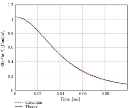
Figure 2 shows the evolution of the charge density distribution function. The solid line shows the theoretical graph and the dotted line shows the graph obtained nu- merically. It should be noted that the solution (2) doesn’t depend on the coordinates, only on time. Therefore, at every time step within the sphere the density is indepen- dent of the radius and remains constant, i.e., it depends only on time. Therefore, in Figure 2 there is no depen- dence on the coordinates, i.e. the value of density can correspond to any point within the sphere. As follows from the graph in Figure 2 there is a good agreement be- tween the theory and the numerical solution obtained by the schemes in Equations (4) and (5), which has a first order approximation in time.

Figure 3 shows the configuration space for PP (Par- ticle-to-Particle) method. On the left we can see the dis- tribution of the particles at the initial time, and on the right—the final position of the particles. The figure shows the volumetric expansion of the sphere.

Let us analyze the behavior of the system of charged particles in the case of a non-uniform charge density. Let us consider a charged sphere with charge density distri- bution function in the form of:

( )

( ( ) )

( )

( )

2 2

ln 2

2

1

e , 2

2 2

r

n p n

q

r r N r

r r

µ σ

ρ ρ ρ

σ

− −

= =

π

π , (7)

where ρn

( )

r is a normal logarithmic distribution;

,

σ µ are constants. As initial conditions, we take the following values:

( )

( )

( )

[ ]

2

0 0 2

0

1000, 0, 0.2

, d

0,1 , 200, 0.01 , 400

p

r r

R T

N м

t r s s s

r

r м N T с N

µ σ

ρ

= = =

= =

∈ = = =

∫

e

V Θ D (8)

The solution of the problem will be sought in two ways: by the numerical solution of the Cauchy problem (1) using the algorithm (4-5) and by the PP (Particle-to- Particle) method. At the end of the calculations the two results are compared.

Suppose there is a three-dimensional area in which the problem is to be solved. To define the area, we take a pa- rallelepiped with side lengths , 1, 2,3

s x

Figure 2. The evolution of the charge density distribution function for a uniformly charged sphere.

gular mesh

{

i j k, ,

}

= ≤ ≤

{

1 i Nx1−1, 1≤ ≤j Nx2−1, 1≤ ≤k Nx3−1

}

(9)

in increments of s

s s x x x L h N

= , where Nx_s is the number

of partitions of Lx_s. We set a time mesh0≤ ≤n NT −1

in increments of τ =T N_T , where T is a period of time, in which the problem is to be solved. The system of difference equations (4) takes on the form:

( ) ( ) ( )

(

)

( ) ( ) ( ) ( ) ( ) ( ) ( ) ( ) ( ) 1 1 1 3 2 2 2

, , , 1 , , , , , , , , , 3

1 2 3

, , , 1 , , , , , , , , , 0

1, , , 1, , , , , ,

, 1, , , 1, , , , 1,

,

, , , 1, 2, 3

2

2

s s s

s s s s

x x x

i j k n i j k n i j k n i j k n

x x x x

i j k n i j k n i j k n i j k n

x x

i j k n i j k n i j k n

x

x

x x

i j k n i j k n i j k n

x

D D V

x x x R s

V V D dV

D D

h

D D D

h τρ α τ ε ρ + + + − + − + = − ∈ =   = +  −    − = − + + ( ) ( ) ( ) ( ) ( ) ( ) ( ) ( ) 3 3 3 1 2

, , 1,

, , , , , , , , , , , , , , , , , , , , ,

2

1 2 3

s s s s

x i j k n

x

x x x x x x x

i j k n i j k n i j k n i j k n i j k n i j k n i j k n D

h

dV V w V w V w

− −

= + +

(10) where the expressions 1( ), , , , 2( ), , , , 3( ), , ,

s s s

x x x

i j k n i j k n i j k n

w w w are de-

rived from the velocity and are determined in accordance with the formulas:

( ) ( ) ( ) ( ) ( ) ( )

( ) ( ) ( )

1 2

3

1, , , 1, , , , 1, , , 1, ,

, , , , , ,

, , 1, , , 1, , , ,

, 2 ,

2 2

3

2

1

s s s s

s s

s s

s

x x x x

i j k n i j k n i j k n i j k n

x x

i j k n i j k n

x x

x x

i j k n i j k n x

i j k n

x

V V V V

w w h h V V w h + − + − + − − − = = − = (11)

(a) (b)

Figure 3. The configuration space of the initial and final particle distribution for the model of a sphere with a con- stant density.

Finding a solution is as follows. First, we set the initial distribution ( ), , ,0

s x i j k

D and ( )_{, , ,0}xs i j k

V , where

{

i j k, ,

}

=

{

0≤ ≤i Nx₁, 0≤ ≤j Nx₂, 0≤ ≤k Nx₃

}

. N e x t ,

using the formulas (10) and (11) we define ( ), , ,1 s x i j k

D and

( )

, , ,1 s x i j k

V in the nodes of the mesh (9). Using the boundary conditions on the surface S or the conditions of sym- metry of the problem, we find the missing values ( ), , ,1

s x i j k D and ( ), , ,1

s x i j k

V in the nodes of the mesh

{

i j k, ,

}

= =

{

i 0,Nx₁,j=0,Nx₂,k=0,Nx₃

}

. Similarly, we

find the value of ( ), , , s x i j k n

D and ( ), , , s x i j k n

V mesh functions on the next layers while n>1.

The difference schemes in Equations (10) and (11) can be applied to the functions with a smooth front. In the case of a discontinuous front another difference scheme adapted to this case must be used.

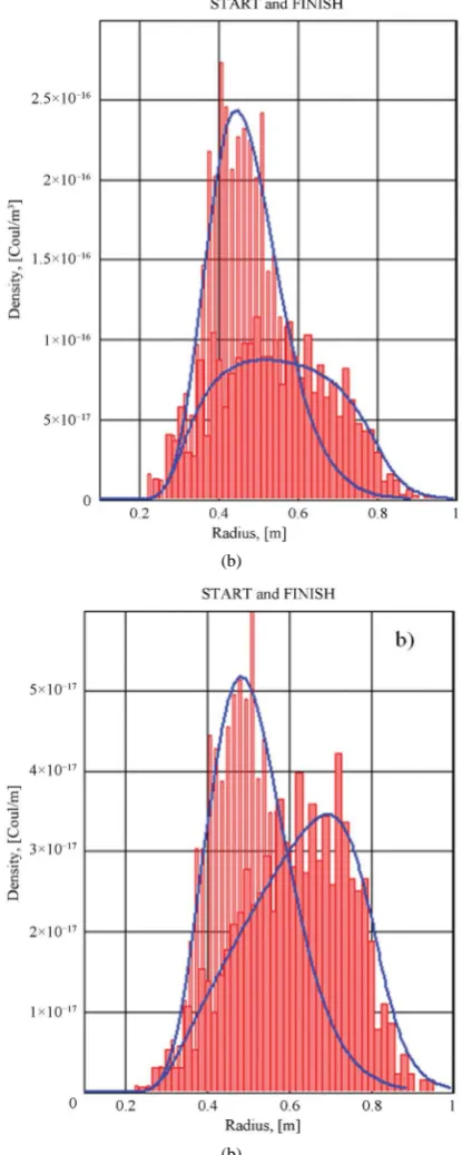
Figures 1(a) and (b) shows the initial and final charge density function distribution along the radius. The solid line shows the density function obtained by solving the problem (1) using the difference schemes in Equations (10) and (11). The bar chart shows the particle density to be calculated by PP (Particle-to-Particle) method. Figure 4(a) shows the function ρ

( )

r , and Figure 4(b) shows the function ρ

( )

r r2. The area under the curve ρ

( )

r r2 corresponds to the total charge of the system, which should remain constant.

A comparison of the distributions in Figure 4 shows that the Cauchy problem (1) and PP method have similar nature of the evolution of the charge density distribution function.

Figure 5 shows the evolution of the charge density distribution function at regular intervals for the Cauchy problem (1). We can see how the spreading of the spher- ical layer of the charge occurs.

[image:4.595.70.278.92.266.2] [image:4.595.309.539.96.216.2]

(b)

(b)

Figure 4. The initial and final distribution of the volume density of the particles for the model of the sphere with a normal logarithmic distribution of the charge density.

4. Conclusion

[image:5.595.312.535.94.219.2]

In this paper, we considered the model solution of the Cauchy problem (1), with the zero initial velocity, and without external fields for the uniform and non-uniform distribution of the charge density. The results of the com-

Figure 5. The dependence of the distribution function of the charge density of the particles on time.

(a)

[image:5.595.68.276.99.619.2]

(b)

Figure 6. The initial and final charge density distribution in the median plane.

parison of the calculations made by using the Particle-to- Particle (PP) method with calculations derived from the numerical solution of the Cauchy problem (1) are shown. The comparison showed a good agreement between the results. Thus, we tested the parameters of the Particle-to- Particle method, which is used in the real problems asso- ciated with the calculation of the space charge effect, for example, in accelerating installations. It is shown that there is a good correspondence to the theoretical data for the uniform case, for which there is an exact solution.

Acknowledgements

[image:5.595.326.522.260.523.2]

in preparation of this manuscript.

REFERENCES

[1] V. P. Maslov, “Equations of the Self-Consistent Field,” Ito- gi Nauki i Tekhniki, Sovremennye Problemy Matematiki, Vol. 11, VINITI, Moscow, 1978, pp. 153-234.

[2] A. A. Vlasov, “Statistical Distribution Functions,” Nauka, Moscow, 1968.

[3] N. G. Inozemtseva and B. I. Sadovnikov, “Evolution of Bo-

golyubov’s Functional Hypothesis,” Physics of Particles and Nuclei, Vol. 18, No. 4, 1987, p. 53.

[4] F. H. Harlow, “The Particle-in-Cell Method for Numeri- cal Solution of Problems in Fluid Dynamics,” Proceed- ings of Symposium in Applied Mathematics, Vol. 15, No. 10, 1963, p. 269.