http://dx.doi.org/10.4236/ojs.2013.36051
High-Dimensional Regression on Sparse Grids
Applied to Pricing Moving Window Asian Options
Stefan Dirnstorfer1, Andreas J. Grau1, Rudi Zagst2 1Thetaris GmbH, Munich, Germany
2Technical University Munich, Munich, Germany
Email: [email protected],[email protected], [email protected]
Received July 29,2013; revised August 29, 2013; accepted September 6, 2013
Copyright © 2013 Stefan Dirnstorfer et al. This is an open access article distributed under the Creative Commons Attribution License, which permits unrestricted use, distribution, and reproduction in any medium, provided the original work is properly cited. In accor- dance of the Creative Commons Attribution License all Copyrights © 2013 are reserved for SCIRP and the owner of the intellectual property Stefan Dirnstorfer et al. All Copyright © 2013 are guarded by law and by SCIRP as a guardian.
ABSTRACT
The pricing of moving window Asian option with an early exercise feature is considered a challenging problem in op- tion pricing. The computational challenge lies in the unknown optimal exercise strategy and in the high dimensionality required for approximating the early exercise boundary. We use sparse grid basis functions in the Least Squares Monte Carlo approach to solve this “curse of dimensionality” problem. The resulting algorithm provides a general and con- vergent method for pricing moving window Asian options. The sparse grid technique presented in this paper can be generalized to pricing other high-dimensional, early-exercisable derivatives.
Keywords: Sparse Grid; Regression; Least-Squares Monte Carlo; Moving Window Asian Option
1. Introduction
Methods for pricing a large variety of exotic options have been developed in the past decades. Still, the pricing of high dimensional American-style moving average op- tions remains a challenging task. The price of this type of options depends on the full path of the underlying, not only at the final exercise date but also during the whole period of exercisable times. We consider in this paper the case of an early-exercisable floating-strike moving win- dow Asian option (MWAO) with discrete observations for the computation of the exercise value. The exercise value of the MWAO depends on a moving average of the underlying stock over a period of time.
Carriere [1] first introduces the simulation-based me- thod for solving American-type option valuation prob- lems. A similar but simpler method is presented by Longstaff and Schwartz [2]. Their method is known as the Least Squares Monte Carlo (LSM) method. It uses the least-squares regression method to determine the op- timal exercise strategy. Longstaff and Schwartz also use their LSM method to price an American-Bermuda-Asian option that can be exercised on a specific set of dates after an initial lockout period. Their American-Ber-
muda-Asian option has an arithmetic average of stock prices as the underlying. The pricing problem can be reduced to two dimensions after introducing another variable in the partial differential equation (PDE) to rep-resent the arithmetic average.
The dimension reduction technique as in Longstaff- Schwartz [2] can not be applied for the pricing problem of MWAOs. Since moving averages shift up and down when the underlying prices shift up and down especially when the first observation in the moving window drops out and a new one comes in, the whole history of stock prices is important in determining the optimal exercise strategy of MWAOs. This leads to an arbitrary number of dimensions and presents a computational challenge. Pricing methods for MWAOs have been described by very few authors besides Broadie and Cao [3]. Broadie and Cao price a fixed strike MWAO, using polynomials of underlying asset price and arithmetic average as the regression basis function. Bilger [4] applies the LSM method to price MWAOs. He uses a different choice of
basis functions (i.e. the underlying asset S and a set of
method is based on the binomial tree model and they include up to 6 discrete observations in the averaging
period for their numerical examples. Bernhart et al. [6]
use a truncated Laguerre series expansion to reduce the infinite dimensional dynamics of a moving average pro- cess to a finite dimensional approximation and then ap- ply the LSM algorithm to price the finite-dimensioned moving average American-type options. Their numerical implementations can handle dimensions up to 8, beyond
that their method becomes infeasible. Dai et al. [7] use a
forward shooting grid method to price European and American-style moving average barrier options. The win- dow lengths in their numerical examples range from three or four days to two or three months.
In this paper, we apply an alternative type of basis functions—the sparse grid basis functions—to the simu-lation-based LSM approach for pricing American-style MWAOs. The sparse grid technique overcomes the low-dimension limit associated with full grid discretiza- tions and achieves reasonable accuracy for approximat- ing high-dimensional problems. Instead of using a pre- determined set of basis functions in the least squares re- gressions, the sparse grid basis functions are adaptive to the data—it is more general and considers as many in- formation in the moving window as possible. Using nu- merical examples, we demonstrate the convergence of the pricing algorithms for MWAOs for different numbers of Monte-Carlo paths, different sparse grid levels and a fixed length of observation period of 10 days. Sparse grid is a discretization technique that is designed to circum- vent the “curse of dimensionality” problem in standard grid-based methods for approximating a function. The idea of sparse grid was originally discovered by Smolyak [8] and was rediscovered by Zenger [9] for PDE solu- tions in 1990. Since then, it has been applied to many dif- ferent topics, such as integration [10,11] or Fast Fourier Transform (FFT) [12]. Sparse grids have also been used for finite element PDE solutions by Bungartz [13],
inter-polation by Bathelmann et al. [14], clustering by Garcke et
al. [15], and PDE option pricing by Reisinger [16].
The structure of this paper is as follows: first, we for- mulate the pricing problem of a moving window Asian option and explain why this problem is computationally challenging. This is followed by a brief description of the LSM approach and the sparse grid technique. Finally, we provide some numerical examples for pricing MWAOs with discretely sampled observations using LSM with sparse grid type basis functions.
Throughout this paper, we consider equity options on a single underlying stock in the Black Scholes [17] frame- work.
2. Moving Window Asian Option
MWAO is an American-style option that makes use of
the moving average dynamics of stock prices. Similar to an American option which pays the difference between the current underlying price and a fixed strike, a MWAO pays the difference between current stock price and the floating moving average or the difference between a floating moving average and a fixed strike.
2.1. Continuous Time Version
Before going into the details of an MWAO, we set up the process for the underlying stock. The stock prices are assumed following a geometric Brownian motion (GBM) process
dSt rS ttd S Wtd t, (1)
where is the constant riskless interest rate, r is the
constant stock return volatility and d is the incre-
ment of a standard Wiener process under the risk-neutral
measure. The initial stock price is denoted as 0 and at
time the stock price is t. The value of a MWAO
option written on the stock is denoted in general as ,
or t resp.
W
S
t S
V V V t S
, t
when we stress the dependence onor t. The option value V satisfies the following
Black Scholes PDE
t S
2 2 2
2
1
0.
2 t t
t t
V V V
S rS rV
t S S
(2)
The following American constraint sets a minimum
value for the function . The constraint has to be satis-
fied at each time 0
V
t>t tw, where 0 denotes the set-
up time of the option and denotes a fixed window
length
t
w
t
, t
t,
V t S P A St , (3)
0
1
d , d
w w
t
t t t t
A t S
(4)where P A S
t, t
t
is the payoff of a MWAO from exer-
cise at time . It depends on the stock price t and a
weighted moving average t
S
A of the stock prices. The
moving average At is computed using the weight func-
tion on a window of stock prices ranging from time
w
tt to time . In this paper, we consider the payoff
function t
t, t
max
t t,0P A S A S
. (5)when setting the weight 1 in (4), we have an
equally-weighted arithmetic moving average 1
d . w
t t t t
w
A S
t
Differentiating this expression with respect to time leads to
t
1
d t t t tw d ,
w
S S t
t
where the updating process of At depends not only on
the stock price at time , but also on the stock price at
time w. This is clearly not Markovian. An optimal
exercise strategy performed on the above moving aver- age process
t tt
t
A has to consider t,
w
t t and all stock
prices w in between. Since all the values
are used in computing the moving average t
S S
, >
u u>tt
S t
u
S A, and
t
A in turn determines the MWAO payoff in (3), there
are infinitely many prices involved in the computation of an optimal exercise strategy. This is a challenging infi- nite-dimensional problem in continuous time [6,7].
2.2. Discretizations
To implement the pricing problem for the MWAO, we consider the finite dimensional case with discretely sam- pled observations. Define a set of times
t0 0, , ,t1 tn T
,
with , and t j for . At time
, the value of and V is respectively denoted as
and V .
, 0, ,
i
t i
S
n i <t
<
i j
i
t
t
S
i ti
We consider constant weight t
in defining a dis-cretely sampled moving average At
1, for0, for
t m
t
t m
(6)
where denotes the number of samples used in com-
puting the moving average. Using the weight function
m
t in defining the moving average At, the boundary
condition (3) at times
has the followingdiscretized form 1
, ,
m n
t t
, ,
1
, ,i i m i j i
i
t t t t t
j i m
V S S P i j S S
m
(7)
where the weight function assigns a zero
weight to an initial observation in the moving window and a weight of one to the rest of the observations. With this weight function we have effectively used the past samples to form the moving window. The above condi-
tion holds for , after an initial allowance for the
window length. The dimension of this MWAO problem
equals to the number of discrete samples used in the
averaging window.
i j
m
im
m
Our method for valuing the MWAO uses the discre-
tized process and a quadrature of . The valuation pro-
ceeds backwards in time, starting at the option maturity , where condition (7) holds with equality. Then we solve for the option value at current time
T
, t
V V t S
0
0 .
For short window length and thus low dimensional-
ity, this procedure can be reformulated in a PDE setting and solved numerically. However, due to the “curse of dimensionality”, the PDE method is ineffective for di-
mensions of more than three or four. For window length larger than four, the high dimensional problem has to be solved using approximate representations or special numerical techniques.
m
m
3. Numerical Procedure
The previous sections provided the mathematical formu- lations and discussed the discretization issues related to the MWAO. This section details the numerical methods we use for pricing MWAOs. The algorithm proposed by this paper is effectively a combination of three tech- niques that are well established in their respective fields. The three techniques that we use as a practical tool for valuing a MWAO are Monte Carlo simulation, least squares regression and sparse grids. Especially in quanti- tative finance, sparse grids technique has not yet lived to its full potential. This paper contributes to use sparse grids in solving high-dimensional problems. Since all the three techniques have been documented in full detail by the cited sources, we summarize in the following the main aspects of each technique. Without explicitly men- tioning it, all prices in our computations are discounted prices, meaning that prices are already normalized by the
bank account numeraire. We use , and V to de-
note discounted stock prices, discounted payoffs and discounted option values.
S P
3.1. Monte Carlo Simulation
A standard method that is used when dimensionality causes numerical difficulties is the Monte Carlo simula- tion method. This method alone does not resolve our issue, but provides the framework for our algorithm. We as- sume that the stock price underlying a MWAO follows the GBM process defined in (1). The discretized stock price
process is sampled at the set of discrete times ti so
that each of the realizations j
S , j
1, , s1
with s1 denoting the number of Monte-Carlo paths, has the fol- lowing normalized representation
2
1 1 1
1
1
2 ,
j
i i i i ti
i i
t t t t j j
t t
S S
(8)
where j1
i
t
is drawn from a standardized Normal
dis-tribution.
The price of the MWAO is the expected value of the (discounted) payoff at the optimal stopping time. The optimal stopping time provides a strategy that maximizes the option value without using any information about future stock prices.
3.2. Least Squares
At each exercise time ti, the option holder decides
whether to exercise the option and get the payoff
,imaximize the option value at time , the holder
exercises if ti
V ti
, i ti1P S t V S t,i, (9)
where denotes the expectation taken under the risk
neutral measure. In the LSM approach, the value of
1 ,
i
t i
V S t
is approximated by a function Pe
S t,i
, 1 , .
i
e
i t i
P S t V S t (10)
The value of e
,i
P S t is computed using a least square
regression on many path-realizations i 1 .
The regressions start at one time step before the maturity .
, 1, ,
Stj j s
T
The function is a linear combination of the
basis functions
,
e i
P S t
k
,
i m i
e i
i k k t k
P S t
a S ,,St
. (11)The coefficients are found by minimizing the
-norm i k a 2 L
12
, , , 1, , ,
i m i
i j j j
k k t t ti k
a S S V j s
(12)where ij
t
V is the option value of a Monte Carlo path
realization j
S at time i. The option value
i
t Vtj is
given as the maximum between the estimated continua- tion value and the intrinsic value. A numerically more stable algorithm is to set
1
if , >
,
, else
i i
j e j
t j t
j i
V P S t P S
V
P S t
, i j T T j i t
(13)where the computed is used only in early-
exercise decisions, this avoids the accumulation of ap- proximation errors when stepping backwards in time.
,e j i
P S t
Given the option payoff VTj P
S , at maturitytime, a backward induction dynamic programming me- thod solves for all values
i
j t
V , starting at time and T
iterating back to . Based on the values 0 ,
we compute an estimated option value, known as the in-sample price
0
t Vtj,j1, , s1
0
1
1 1
1 s .
in j
t j
V
s
V (14)This approach has an obvious shortcoming. Each of
the estimated option values 0j
t V , i j t i S t
contains information
about its future stock path . In order to avoid
this perfect foresight bias, we compute an out-of-sample
option price: we generate additional simulation paths ,
but use the coefficients fitted
to the old set of simulation paths
l
S
1 1, , 1l s s s2 aik
j
S , j
1,,s1
. Consequently, the out-of-sample value does not dependon knowledge of the future paths. The out-of-sample option value is computed by
1 2
0 1 1
2
1 s s ,
out l t l s V s
Vl i t (15) with
1if , ,
.
, else
i i
l e l
t i
l t
l i
V P S t P S
V
P S t
(16)
In our implementations, we compute only the out-of- sample value since it is the value for which we can state the optimal exercise policy without information about the future. The expected value of the out-of-sample price
is always a lower bound for the option value, and
the estimate is crucial for the convergence of the
least squares Monte Carlo simulation method. We are confined to finitely many samples and to finite degrees of freedom in the regressions, thus are not able to perfectly represent the real shape of
out V e P 1 i
t i
using the esti-
mate . A less than optimal exercise strategy is per-
formed and provides a lower biased option value. ,
V S t
e P
3.3. Basis Functions
An important issue in the LSM approach is a careful
choice of the basis functions k in (11). We will use in
this paper a linear combination of the sparse grid type basis functions to approximate the conditional expected value Vti1 S t,i involved in the optimal exercise
rules. We need one dimension for each observation in the averaging window, this leads to a high dimensionality in the computational problem. Sparse grid [8] is a discreti-zation technique designed to circumvent this “curse of dimensionality” problem. It gives a more efficient selec-tion of basis funcselec-tions. This technique has been success-fully applied in the field of high-dimensional function approximations [15] and many others [10,13,16,18].
In the following we provide a brief description of the sparse grid approach. We start from constructing one- dimensional basis functions in a general case and show how to build multi-dimensional basis functions from the one-dimensional ones. Next we create a finite set of basis functions for numerical computations. Sparse grid then efficiently combines the sets of basis functions in a way such that the resulting function set is linearly independ- ent. Following this, we detail on two specific types of sparse basis functions - a polynomial function and a piecewise linear function - to be used as the basis func- tions in the LSM regressions in this paper.
3.3.1. Constructing the Basis Functions
mon to build such a function representation using some basis functions. We consider here a set of basis functions
1, , ,2 n
and we call the set (sets) of basis
functions “function basis (bases)”. From the set , we
construct an approximating function f as a linear com-
bination of the basis functions
1
,
n k k k
f x a x
(17)
with coefficients ak for k,k1, , n , and xX
for some set X. The basis functions k
x can be aone-dimensional or multi-dimensional mapping from
to .
X R
For the one-dimensional case, many function bases are well known and widely used. Examples include polyno- mials, splines, B-splines, Bessel functions, trigonometric functions, and so on. For the multi-dimensional case, the set of basis functions that are commonly used is more scarce. There are two common approaches to construct- ing multi-dimensional basis functions from the one-di- mensional ones: the radial basis functions [19] and the tensor product functions [20]. In this paper we focus on the tensor product approach. To construct a tensor product basis function, we select one-dimensional
func-tions and multiply their respective function value
evaluated at the corresponding component of x .
Specifically, for and each m-dimensional basis
function
m
X R
k
, we choose a set of one dimensional
func-tions
k,1, k,2, ,k m,
and
1, , ,2 m
x x x x ,
then multiply the -th function j k j, evaluated at the
-th element j
j x , for , to have the following
representation of an -dimensional basis function
1, ,
j m m
,1
1 ,2
2 ,
.k x k x k x k m xm
(18)
3.3.2. Creating a Function Basis
Having created multi-dimensional basis functions in a general case, we now select a finite set of these functions to be our basis for numerical analyses. Since we will do computations on different levels of accuracy, we will also need a set of basis functions on different levels. Naturally, the more basis functions we put in the set, the more accurate are our function approximations.
We decide that on a level L there are
L 1 ba-sis functions. The one-dimensional function basis L
with
L 1 functions is the following set
1, 2, , 1 ,L L
where i,i
1, ,
L 1
are one-dimensional basisfunctions, and
L is a monotonously increasingfunction that determines the size of our basis at level L.
In order to create an -dimensional function basis,
we choose a level
m
1, , ,L2 Lm
L L . For each dimen-
sion j
1, , m
, the level Lj implies a function ba-sis j
1, 2, , 1
j
L L
via (19). Using the ten-
sor product function, the m-dimensional function basis
L
is constructed as
11,12, ,2 2 , 1, ,
m
j
L L L L
m m j L ,
x x x x j m
(20)
where j
xj denotes any of the one-dimensional ba-
sis functions from Lj, evaluated at the jt element of h
1, , ,2 m
x x x x .
It was our original goal to construct a function basis with increasing expressiveness for increasing levels. This multi-dimensional level is not a very good starting point. Consider the case where all dimensions are equally important, we would have to use a level of the form
L
, , ,
L . The size of the resulting function set would be extremely large, a phenomenon known as the “curse of dimensionality” problem:
, , , . m L
(21)
Choosing m10 dimensions and
3 resultsin functions with a corresponding number of coeffi-
cients to be solved.
10
3
3.3.3. Sparse Grids
Sparse grids were developed as an escape from the “curse of dimensionality” problem. They allow reasona- bly accurate approximations in high dimensions at low computational cost. The idea behind the sparse grid is to combine the tensor basis of different levels.
Let *
L
be the set of basis functions on level .
We define it as the union of all tensor function bases
* L
L
where the sum of levels
isequal to , with and denoting the set of
all non-negative numbers
m
0
0L1L2 Lm
*
L L*
*
*
1 2
1, ,
.
m m
L L
L L L L L L L
(22)Considering a simple example with dimen-
sions on level
2 m
* 2
L , i.e. . For k 0
* 1 2
L L L 2 L
with 1, 2k , there are three possible combi- nations of
the levels L1 and L2 that sum to 2:
0,2 ,
1,1 and
2, 0 . From this, we could create a set * 2L
as the union of the tensor function bases: 2,0 1,1 0,2.
(19) The first set 2,0 has high resolution in the firstdi-mension , while the last set mainly resolves
1
the second dimension 2. By construction, basis
func-tions with high resolution in both dimensions, such as
2,2 , are left out in the sparse set, making the sparse
basis ideal for approximating functions with bounded mixed derivatives.
L
The computational effort of sparse grids compared with conventional full grids decreases radically while the error
rises only slightly: for the representation of a function f
over an m-dimensional domain with minimal mesh
size 2 L
L
h , a sparse grid employs O h
L1 loghLm1
points and a full grid has
mL
O h grid points. At the
same time, the L2 interpolation error for smooth func-
tions is
2 log
L
O h hLm1 for sparse grids and O h
L2for full grids.
Having constructed a sparse basis L* on a top
level, we now create two specific types of sparse basis functions that will be used as the function sets in our LSM regression problem: a polynomial sparse function basis and a piecewise linear function basis. Compared to the piecewise linear basis functions, the polynomial sparse basis functions are easier to understand and eas-ier to implement. As solutions to higher dimensional problems, the piecewise linear basis functions are more adaptive. They can be extended to effectively place the basis functions on the dimension that contributes more to the problem solution. As a result, piecewise linear basis functions have seen wide applicability to solving PDEs [18] and interpolating functions [21]. In our paper, we use these two types of sparse basis functions to cross validate the results of our high dimensional pricing problem.
3.3.4. A Polynomial Sparse Basis
A polynomial function basis with basis func-
tions in the one-dimensional case has the following con- struction
L 1
1, 2, , ,3 L .L x x
x x,
(23)From the one-dimensional functions L, we can
build a multi-dimensional tensor basis according to (20).
As an example, for the two-dimensional case
m2
,we have the first dimension in x with one-dimensional
functions
1
1
2 3
1, , , , L
L x x
x x,
, y y
,
and the second dimension in with one-dimensional functions
y
2
2
2 3
1, , , , L
L y y
.
Equation (20) then gives the following list of tensor basis functions 1 2 1 1
2 2 2 1
, 2 2 2 1 L L L L
L L L L L
x x x
y xy x y x y
y xy x y x y
2 (24)
Building upon the two-dimensional function basis
L L1, 2, we construct a sparse basis function set for the
three sparse levels
* 0
L , L*1, and L*2, where
*
L L1L2. We let the three levels correspond to
*
L
0 0,
*= 1 =
L 2
and
*
6L
2 num-
ber of basis functions. Using (22) to unite the function sets, our sparse bases for the two dimensional function space are the following sets
* * * 0,0 0 2 2 1,0 0,1 1 2 22,0 1,1 0,2 2
2 3 4 5 6 2 3 4
5 6 2 2 2 2
1
1, , 1, ,
1, , , ,
1, , , , , , , , , , ,
, , , , , . poly L poly L poly L
x x y y
x x y y
x x x x x x y y y y
y y xy x y xy x y
(25)
The above sparse basis function sets *
poly L
are cre-
ated by taking the unions of the tensor bases of
1,2
L L
according to (22). As an example, the sparse set *1
poly L
is constructed as a union of
1 2
2 1,0 L1,L0 1, ,x x
and
1 2
2 0,1 L0,L 1 1, ,y y
.
The set 1,0 is arrived at by having
L1 1
2number of basis functions in the x direction and
L2 0
0 basis functions in the direction from
the two-dimensional set
y
L L1, 2
We have just created a polynomial sparse basis *
, ceteris paribus.
poly
L
in two dimensions. Higher dimensional function bases can be similarly constructed using the tensor product approach, depending on the dimension of the problem we intend to solve. In our LSM regression problems, we
have for example used m10 dimensions and a poly-
nomial sparse level of *
0,1,2
L .
3.3.5. Piecewise Linear Functions on [0,1] It has been found computationally advisable to have
only one basis function on the first level. Hence we start
with the constant 1 on level * 0 and transform
L
on successive levels. This construction avoids the inclu- sion of costly boundary points by creating boundary func- tions that are less scaled than inner functions. Klimke and Wohlmuth [21] is a good reference on piecewise linear basis functions.
The piecewise linear function is a type of basis function that is commonly used in sparse grid applications. To create a piecewise basis for various levels, we utilize a construction approach known from multi-resolution
analysis. We define a mother function
x and gen-erate our basis by scaling and translating from
x
1 when 1,0
1 when 0,1
0 otherwise
x x
x x x
(26)
The one-dimensional function bases of levels L10,
1 1
L , L12,
, L1k in x as generated fromthe one-dimensional basis functions in (26) are the
following sets
1 1 1 1 1 0 1 0 2 1 12 , 2 2
4 , 4 4 8 3 , 8 5
L
L L
L L
x x
x x x x
(27)
1 1 1
1 1 1 1 1
2 , 2 2
2 3 , 2 5 , 2 7 , , 2 2 3
k k k
L k L k
k k k k k
x x
x x x x
, (28)where the series 3,5,7, , 2
k13
in (28) is a se-quence of odd numbers. The one-dimensional function
bases in y can be analogously generated from (26).
The construction of a two-dimensional sparse basis in
the x and directions respectively for levels y L*0,
L* = 1 and L*2, where L* L1L2, follows from (22)
* * * 0,0 0 1,0 0,1 12,0 1,1 0,2 2
1
1, 2 , 2 2 , 2 , 2 2
1, 2 , 2 2 , 4 , 4 4 , 8 3 , 8 5 , 2 , 2 2 , 4 ,
4 4 , 8 3 , 8 5 , 2 2 , 2 2 2 , 2 2 2 ,
2 2 2 2 .
piece L piece L piece L
x x y y
x x x x x x y y
y y y x y x y x y
x y y (29)
As an example, the sparse basis function set * 2
piece L
is
created by taking the unions of the function bases of
2,0
, 1,1 , and 0,2 , where
1 2
2,0 L2,L0
is
the tensor product of L12 and L20, with L12
given in (27) and L20 1. The set L L1,2 is con-
structed using the tensor product function (20).
The two-dimensional sparse bases can be extended to higher dimensions depending on the problem dimensions we intend to solve. The resulting higher-dimensional function sets can then be used in the LSM regressions by selecting an optimal sparse level for that problem dimen- sion.
3.3.6. Implementations
We perform the regressions required by (12) on sparse
polynomial basis functions poly*
L
and sparse piecewise
linear basis functions *
piece
L as explained in Section
3.3.4 and 3.3.5, respectively. As an example, in the case
of sparse polynomial basis functions of dimen-
sions, the approximating function of (11) is a linear
combination of the basis functions in the polynomial sparse basis set
2 m e P * poly L
in (25). At sparse level * 1
L ,
2
1, ,2 2 1
poly L
the set * 1, ,x x x x1 2
1 2 4 2 i i i j a a a x
, and the approximating
function
,
e j i
t
1 2. j x
3 2 2 i jP x x
x 1 5 j i a a
For the sparse piecewise linear basis functions of 2
m dimensions, the approximating function is a
linear combination of the basis functions in the piecewise linear sparse basis set
e P
*
piece L
* 1 L
* 1
piec L
0
j
, the set
1, 2 1 , 2 1 2 , 2 2 , 2 2 2
e
x x x x
,
and the approximating function
1 2 1 3 1
4 2 5 2
, 2 2
2 2 2
e j i i j i j
i
i j i j
P x t a a x a x
a x a x
2
m
In our implementations, we use sparse levels from
up to 3 and dimensions for computing the
basis functions. This is sufficient for our purposes. But, we do not perform the regressions on directly. In-
stead, we use scaled values of such that for each path
, we compute
* L
10
m
S
S
1, , 1
1 i, , 1 i
j j j j j j j
m t m t
x x x S S ,
where
1j, , j
m
1 are defined such that j
0,1m1x .
For discretely sampled observations, the dimension of
the problem is effectively dimensions because of the
weight function
m
used in computing the moving av-
erages. When extrapolating to the continuous case, the dimension of the problem approaches infinity as
goes to .
m
The regression itself is performed solving the least squares problem of (12) via QR-decomposition. Fur- thermore, the regression is only performed on paths with
a positive exercise value . This sig-
nificantly decreases the computational effort.
: , >
j j
i
S P S t 0
4. Numerical Example
We provide in this section a numerical case study of us- ing sparse grid basis functions in LSM pricing MWAOs. We will use a discretely sampled averaging window
spanning ten observations with the weight function α in
(6).
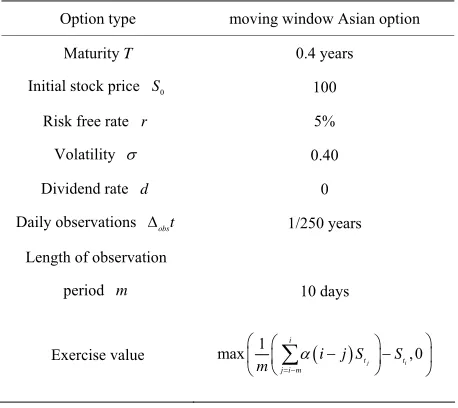
The properties of the MWAO are defined in Table 1.
The underlying stock prices are sampled at a regular fre-quency, e.g. every trading day at a specific time.
To analyze the convergence of our pricing algorithm
for MWAOs, we use the notation i
, ,*
V n L m to de-
note the out-of-sample result as defined in (15).
Each Monte Carlo value
out V
, ,*
Vi n L m
n
depends on the number of sample paths , the level of the sparse grid function basis , the number of observations in the
averaging window , and the quadrature scheme
* L
m .
We compute different Vi
n L m, ,*
with , n L*, m
and fixed in order to get an estimate for the mean
*
1
1
, , I i , ,
i
V n L m V n L m
I
*
(30)of I different Monte Carlo prices. Each valua-
tion
iI
i
, ,*
[image:8.595.309.538.122.326.2]V n L m is based on a randomly generated
Table 1. Specifications of a moving window Asian option with a floating strike. The moving averages are based on discretely sampled stock prices.
Option type moving window Asian option
Maturity T 0.4 years
Initial stock price S0 100
Risk free rate r 5%
Volatility 0.40 Dividend rate d 0 Daily observations obst 1/250 years
Length of observation
period m 10 days
Exercise value max 1 ,0
j i
i
t t
j i m
i j S S
m
Monte Carlo seed. The number of I ranges from 10 to
1000 depending on an estimate of the Monte Carlo error. For instance, if the error is acceptable based on our 95%
confidence level at I10, we stop the computation and
obtain the mean price estimate using (30). Otherwise, we
continue computing i
, ,L*
V n m by increasing the
value of I until the error is acceptable. The number of
samples per Monte Carlo price results from combin-
ing the in-sample paths
n
1
, ,
1 s
S
2
S and the out-of-sam-
ple paths s1 1, , s1 s
S
S such that 1 2. We use
30% of the sample paths for regressions and 70% for option valuation out-of-sample.
n s s
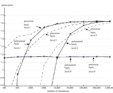
Figure 1 presents the mean V
n L, ,10*
for differ-ent numbers of samples and different levels , but with the dimensions
n
10
* L
m and the weights fixed.
Included in the figure are the results from the polynomial and the piecewise linear sparse basis functions. The op-
tion values at sparse level converge quickly to a
value of about
*= 0 L
7.17
m
V which does not change after
30,000 simulations. With , the sparse level
consists of just one basis function (i.e. a constant) and the
resulting exercising decision is almost trivial. Sparse level
10
0
* 1
L consists of 21 basis functions. This allows
for a more sophisticated strategy with a better utilization of the option. After about 300,000 simulations, the option value saturates at 7.62 for both polynomial and piecewise
linear basis functions. The sparse level with 241
basis functions results in similar values after 1,000,000 simulations. For the polynomial sparse basis functions, a third level
* 2 L
* 3
L with 2001 basis functions already
100 300 1000 3000 10,000 30,000 100,000 300,000 1,000,000 number of simulations
6.8 6.9 7 7.1 7.2 7.3 7.4 7.5 7.6 7.7
option price
piecewise basis level 0 piecewise
basis level 2 piecewise
basis
level 1 piecewise
basis level 3
polynomial basis level 2
polynomial basis level 0 basis
[image:9.595.109.484.76.385.2]level 1 polynomial
Figure 1. The option values for MWAO. The figure shows MWAO values estimated by least squares Monte Carlo combined respectively with polynomial sparse basis functions and with piecewise linear sparse basis functions. The sparse level ranges from 0 to 3 and the number of simulation paths runs from to . In the figure, “polynomial basis level #” refers to the MWAO values estimated with the polynomial basis functions at a sparse level #, where # is the number for the sparse level. Similarly, “piecewise basis level #” points to MWAO values estimated with the piecewise linear basis functions at the sparse level #. The data for the MWAO are specified in Table 1.
2
1 10 6
1 10
thing worth mentioning is that higher sparse levels ini- tially perform inferior to lower sparse levels due to the over-fitted regression functions.
The corresponding values in Figure 1 are presented in
Table 2 for polynomial sparse basis functions and in Table 3 for piecewise linear sparse basis functions. The
mean values of a series of valuations i
, ,10*
,V n L 1, ,
i I, is denoted by V
n L, ,10*
(30), the stan-dard deviation of the series across I valuations is de-
noted by ˆ. For a single evaluation with
LSM,
i
, ,10*V n L
ˆ
can be seen as a measure of how close the
value is to the mean of I valuations. Thus ˆ does not
measure the error relative to the true option value. The
mean estimate
, ,*
L 10
V n (30) will be biased lower
than the true values due to the suboptimal estimate of the
optimal exercise strategy 1
i
t ,ti
V S
. At sparse level
both polynomial and piecewise linear basis func- tions deliver similar MWAO prices up to two decimal
points after sample paths. At sparse level
* 1 L
5
3 10 *
L 2
with sample paths the MWAO prices are the
same up to three decimal point in both cases. Based on the results, both types of sparse basis functions solve our
high-dimensional least squares problem and the prices
converge to a level of at sample paths for
sparse levels
6
0 1 1
7.62 1 10 6
* 1
L and sparse level . Since the
polynomial sparse basis functions are easier to construct and easier to implement, we recommend them as the bases of choice for our MWAO pricing problem.
* 2 L
L
The price of our moving average window option has three main sources of error: the number of simulation
paths , the level of the function basis and the
number of integration samples . The best possible
approximation would have to reduce the errors originated from using these limiting parameters.
n *
m
5. Conclusion
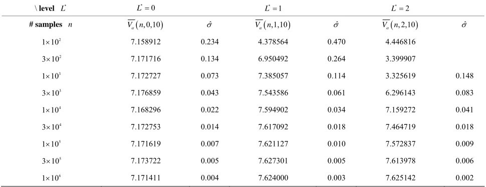
Table 2. The option value for MWAO with data in Table 1 estimated by least squares Monte Carlo with polynomial sparse basis functions. The mean estimate
, ,*10
α
V n L
(30) is based on sample , sparse level , number of observations in the averaging window , and the weight functionn L*
10
m . The number of samples ranges from to , and the
sparse level goes from 0 to . The standard deviation of the series
n 2
1 10 6
1 10
*
L 2
, ,*
10 L i α
V n is denoted by ˆ. \ level L* L*0 * 1
L L*2
# samples n Vn,0,10 ˆ Vn,1,10 ˆ Vn, 2,10 ˆ
2
1 10 7.158912 0.234 4.378564 0.470 4.446816
2
3 10 7.171716 0.134 6.950492 0.264 3.399907
3
1 10 7.172727 0.073 7.385057 0.114 3.325619 0.148
3
3 10 7.176859 0.043 7.543586 0.061 6.296143 0.083
4
1 10 7.168296 0.022 7.594902 0.034 7.159272 0.041
4
3 10 7.172753 0.014 7.617092 0.018 7.464719 0.018
5
1 10 7.171619 0.007 7.621127 0.010 7.572837 0.009
5
3 10 7.173722 0.005 7.627301 0.005 7.613978 0.006
6
[image:10.595.55.540.153.340.2] [image:10.595.61.540.417.605.2]1 10 7.171411 0.004 7.624000 0.003 7.625142 0.002
Table 3. The option value for MWAO with data in Table 1 estimated by least squares Monte Carlo with piecewise linear sparse basis functions. The mean estimate
, ,*10
α
V n L
(30) is based on sample , sparse level , number of observations in the averaging window , and the weight functionn L*
10
m . The number of samples ranges from to ,
and the sparse level goes from 0 to . The standard deviation of the series
n 2
1 10 6
1 10
*
L 3 V
n, ,*
10 L i
α is denoted by ˆ.
\ level L* L*0 * 1
L L*2 L*= 3
# samples n Vn,0,10 ˆ Vn,1,10 ˆ Vn, 2,10 ˆ V n ,3,10 ˆ
2
1 10 7.157866 0.257 7.271832 0.293 6.527391 0.427 5.631500 0.468 2
3 10 7.171375 0.172 7.432182 0.146 7.035495 0.154 6.130585 0.240 3
1 10 7.172456 0.062 7.459452 0.094 7.306664 0.080 6.103082 0.354 3
3 10 7.176906 0.050 7.555757 0.052 7.459485 0.051 7.067918 0.077 4
1 10 7.168270 0.029 7.586647 0.046 7.521104 0.043 7.313780 0.036 4
3 10 7.172753 0.016 7.614570 0.020 7.576200 0.019 7.444699 0.021 5
1 10 7.171629 0.009 7.617702 0.012 7.601458 0.011 7.524500 0.010 5
3 10 7.173733 0.005 7.624306 0.007 7.621602 0.007 7.578699 0.006 6
1 10 7.171410 0.003 7.621104 0.004 7.625030 0.004 7.606029 0.004
sparse grid basis functions. The sparse grid technique has been specifically developed as a cure to the “curse of dimensionality” problem. It allows more efficient selec- tion of basis functions and can successfully approximate high-dimensional functions with less computational ef- fort. We have used both the polynomial and the piece- wise linear sparse basis functions in the least-squares regressions and found that the results converge to values up to two decimal points, independent of the type of ba- sis functions used. We recommend the polynomial sparse
basis as the basis of choice for this type of pricing prob- lems since they are easier to construct and easier to im- plement. The approach presented in this paper can be generalized to pricing other high-dimensional early-ex- ercisable derivatives that use a moving average as the underlying.
REFERENCES
liptic Partial Differential Equations with Variable Coef- ficients,” Computing, Vol. 71, No. 1, 2003, pp. 1-15. http://dx.doi.org/10.1007/s00607-003-0012-8
[2] V. Bathelmann, E. Novak and K. Ritter, “High Dimen- sional Polynomial Interpolation on Sparse Grids,” Ad- vances in Compuational Mathematics, Vol. 12, No. 4, 2000, pp. 273-288.
http://dx.doi.org/10.1023/A:1018977404843
[3] M. Bernhart, P. Tankov and X. Warin, “A Finite Di- mensional Approximation for Pricing Moving Average Options,” Journal on Financial Mathematics, Vol. 2, No. 1, 2011, pp. 989-1013.
http://dx.doi.org/10.1137/100815566
[4] R. Bilger, “Valuing American-Asian Options Using the Longstaff-Schwartz Algorithm,” Msc Thesis in Compu- tational Finance, Oxford University, Oxford, 2003. [5] F. Black and M. Scholes, “The Pricing Of Options and
Corporate Liabilities,” Journal on Political Economy, Vol. 81, No. 3, 1973, pp. 637-659.
http://dx.doi.org/10.1086/260062
[6] T. Bonk, “A New Algorithm for Multi-Dimensional Adaptic Numerical Quadrature,” In: W. Hackbush, Ed., Adaptive Methods—Algorithms, Theory and Applications, Notes on Numerical Fluid Mechanics, Vieweg + Teubner, Brauns- chweig, 1994, pp. 54-68.
[7] M. Broadie and M. Cao, “Improved Lower and Upper Bound Algorithms for Pricing American Options by Simulation,” Quantitative Finance, Vol. 8, No. 8, 2008, pp. 845-861.
http://dx.doi.org/10.1080/14697680701763086
[8] H.-J. Bungartz, “A Multigrid Algorithm for Higher Order Finite Elements on Sparse Grid,” Electronic Transactions on Numerical Analysis, Vol. 6, 1997, pp. 63-77.
[9] J. F. Carriere, “Valuation of the Early-Exercise Price for Options Using Simulations and Nonparametric Regres- sion,” Insurance: Mathematics and Economics, Vol. 19, No. 1, 1996, pp. 19-30.
http://dx.doi.org/10.1016/S0167-6687(96)00004-2 [10] M. Dai, P. Li and J. E. Zhang, “A Lattice Algorithm for
Pricing Moving Average Barrier Options,” Journal of Economic Dynamics and Control, Vol. 34, No. 3, 2010, pp. 542-554. http://dx.doi.org/10.1016/j.jedc.2009.10.008 [11] S. Dirnstorfer, A. J. Grau and H. Li, “ThetaML Hand-
book,” edition winterwork, 2012.
[12] S. Dirnstorfer and A. J. Grau, “Computer Aided Finance: Another Journey in the Quest for the Holy Grail of Fi-
nancial Engineering,” WILMOTT Magazine, 2008, pp. 68-73.
[13] J. Garcke, M. Griebel and M. Thess, “Data Mining with Sparse Grids,” Computing, Vol. 67, No. 3, 2001, pp. 225- 253. http://dx.doi.org/10.1007/s006070170007
[14] K. Hallatschek, “Fouriertransformation auf Dünnen Gittern mit Hierarchischen Basen,” Numerische Mathematik, Vol. 63, No. 1, 1992, pp. 83-97.
http://dx.doi.org/10.1007/BF01385849
[15] C.-H. Kao and Y.-D. Lyuu, “Pricing of Moving Average- Type Options with Applications,” Journal of Futures Markets, Vol. 23, No. 5, 2003, pp. 415-440.
http://dx.doi.org/10.1002/fut.10072
[16] A. Klimke and B. Wohlmuth, “Algorithm 847: Spinterp: Piecewise Multilinear Hierarchical Sparse Grid Interpo- lation in Matlab,” ACM Transactions on Mathematical Software, Vol. 31, No. 4, 2005, pp. 561-579.
http://dx.doi.org/10.1145/1114268.1114275
[17] F. A. Longstaff and E. S. Schwartz, “Valuing American Options by Simulation—A Simple Least-Squares Ap- proach,” The Review of Financial Studies, Vol. 14, No. 1, 2001, pp. 113-147. http://dx.doi.org/10.1093/rfs/14.1.113 [18] B. D. Martin, “Radial Basis Functions: Theory and Im-
plementations,” Cambridge University Press, Cambridge, 2003.
[19] M. Griebel, P. Oswald and T. Schiekoffer, “Sparse Grids for Boundary Integral Equations,” Numerische Mathe- matik, Vol. 83, No. 2, 1999, pp. 279-312.
http://dx.doi.org/10.1007/s002110050450
[20] B. Nicolas, “Elements of Mathematics, Algebra I,” Springer- Verlag, Berlin, 1989.
[21] C. Reisinger, “Numerische Methoden für Hochdimensionale Parabolische Gleichungen am Beispiel von Optionsprei- saufgaben,” Dissertation, Ruprecht-Karls-Universität, Heidel- berg, 2004.
[22] S. Schraufstetter, “A Pricing Framework for the Efficient Evaluation of Financial Derivatives Based on Theta Cal- culus and Adaptive Sparse Grids,” Dr. Hut, 2012. [23] S. A. Smolyak, “Quadrature and Interpolation Formulas
for Tensor Products of Certain Classes of Functions,” Doklady Akademii Nauk SSSR, Vol. 148, 1963, pp. 1042- 1043. English Russian Translation: Soviet Mathematics Doklady, Vol. 4, 1963, pp. 240-243.
Appendix
ThetaML Implementation of the MWAO
This appendix gives a ThetaML (Theta Modeling Lan-
guage)1 implementation of the MWAO pricing problem
described in the text. To help understand the code, we first provide a brief description of the ThetaML language and some ThetaML specific commands and operators used in the models.
ThetaML supports standard control structures such as loops and if statements. It operates on a virtual timing
model with the theta command. The theta command de-
scribes the time-determined behavior of financial deriva-
tives. It allows time to pass. The fork command makes it
possible to model simultaneous processes and enables cross-dependencies among the stochastic variables. The
future operator “!” allows forward access to the future values of a variable, this operation is based on forward algorithms.
ThetaML modularizes the pricing task of MWAO into a simulation model for the stock prices and the numeraire, an exercise model for obtaining future early-exercise values, and a pricing model for computing the MWAO prices. ThetaML virtually parallels and synchronizes the processes—stock prices, numeraire, early exercise cash flows and MWAO prices—to the effect that it is as if these four processes step forward in time as they would have behaved in real life financial markets. ThetaML specific commands and operators are briefly explained in the models where they appear. Process variables in ThetaML models, such as “S”, “CUR”, “A”, implicitly incorporates scenario- and time-indices.
1 model StateProcesses
2 % This model simulates stock prices that follow a Geometric Brownian motion process, 3 % and a numeraire process that are discounted at a constant interest rate;
4 % the arguments are in troduced into the model after the “import” keyword, results 5 % computed by the model are exported
6 import S0 “Initial stock prices” 7 import r “Risk_free interest rate” 8 import sigma “Volatility of stock prices” 9 export S “Stock price process”
10 export CUR “Numeraire process in currency CUR” 11
12 % initialize the stock prices at “S0” 13 S = S0
14 % initialize the numeraire at 1 CUR 15 CUR = 1
16 % “loop inf” runs till the expiry time of a pricing application 17 loop inf
18 % “@dt” extracts the smallest time interval from this model time to the next 19 theta @dt
20 % updates the GBM process of the stock prices for the time step “@dt” 21 S = S * exp((r - 0.5*sigma^2)*@dt + sigma*sqrt(@dt)*randn()) 22 % update the numeraire for the time step “@dt”
23 CUR = CUR*exp(-r*@dt) 24 end
25 end
1 model MWAOExerciseValue
2 % This model computes the Early exercise values for MWAO, assuming daily exercises. 3 % Early exercises are possible after an initial allowance of a window length “m” 4 import S “Stock prices”
5 import CUR “Numeraire in currency CUR” 6 import m “Window length”
7 import T “Option maturity time” 8 export ExerciseValue “Exercise value”
9 export TimeGrid “A set of exercise times”
*ThetaML is a payoff description language that explicitly incorporates the passage of time. Product path dependencies, settlements, and early
10
11 % initialize an array with length “m” to hold a past window of “m” stock prices 12 C = 0 * [1:m]
13 % initialize the moving average to “S/m”, where “S” are the time 0 stock prices 14 A = S/m
15 % initialize “C[m]” to the time 0 stock prices “S” 16 C[m] = S
17
18 ExerciseValue = 0 19 index = 1
20 % early exercise times range from “1/250” to “T”, equally spaced at “1/250” 21 TimeGrid = [1/250:1/250:T]
22
23 % “t” loops through the exercise time sand takes the value of the pointed element 24 loop t: Time Grid
25 % “theta” advances “t_@time” time units to the next time point 26 theta t_@time
27 % update the moving average by adding “S” evaluated at this time divided by “m”; 28 % at the end of “m” periods, subtract “S/m” evaluated at the start window time 29 A = A + S/m - C[index]/m
30 % record the stock price “S” at this time in “C” 31 C[index] = S
32 % increment the index by 1 33 index = index + 1
34 % reset “index” to 1 if “index” is bigger than “m” 35 if index > m
36 index = 1 37 end
38
39 % store the discounted exercise values for in-the-money paths 40 if @time >= 1/250 * (m-1)
41 ExerciseValue = max(A-S,0)*CUR 42 end
43
44 theta @dt
45 % reset Exercise Value to 0 at non-exercising times 46 ExerciseValue = 0
47
48 end 49 end
1 model MWAOPrice
2 % This model returns the MWAO prices across all the Monte-Carlo paths, using the 3 % early-exercise strategies obtained from the model MWAO Exercise Values 4 import Exercise Value “Exercise value”
5 import TimeGrid “A set of exercise times” 6 export Price “MWAO prices”
7
8 % at time 0, “Price” is assigned expected value of “value!”; the future operator “!” accesses the 9 % values of the variable “value” determine data later in stance
10 Price = E(value!)
11 % loop through the exercise times 12 loop t: TimeGrid
16 if E(value!) < ExerciseValue 17 value = ExerciseValue 18 end
19 % time passing of “t-@time” with the “theta” command 20 theta t-@ time
21 end
22 % at the option maturity time, set the option pay off values 23 if ExerciseValue>0
24 value = ExerciseValue 25 else
26 value = 0 27 end
28 end
The stock prices and numeraire are first simulated in the external models “StateProcesses”, then imported as processes into the exercise model “MWAOExercise Values” to compute future early-exercise values. The early-exercise cash flows are next imported as a process into the pricing model “MWAOPrice” to determine the MWAO price.
The ThetaML future operator “!” appears in the model