HARDWARE IMPLEMENTATION OF SATELLITE IMAGE COMPRESSION FILTER USING LIFTING BASED5/3 WAVELETS

ISSN: 1992-8645 www.jatit.org E-ISSN: 1817-3195

347

CLASSIFICATION OF DRIVER FATIGUE STATE BASED ON

EEG USING EMOTIV EPOC+

1

Brilian T. Nugraha, 2 Riyanarto Sarno, 3 Dimas Anton Asfani, 4 Tomohiko Igasaki, 5 M. Nadzeri Munawar

1 2 5

Department of Informatics, Institut Teknologi Sepuluh Nopember, Indonesia

3

Department of Electrical Engineering, Institut Teknologi Sepuluh Nopember, Indonesia

4

School of Science and Technology, Kumamoto University, Japan

E-mail: [email protected], [email protected], [email protected],

4

[email protected], [email protected]

ABSTRACT

Driver fatigue is a major issue since many people have been aware about safety degree of driving. In this regard, this paper proposes methods and application to determine the driving fatigue state for every 3 minutes. The collected EEG data come from 30 participants that were taken their EEG data using Emotiv EPOC+ with the duration of 33 or 60 minutes during driving simulation and their answers about the driving fatigue states for every 3 minutes. The participant and channel outliers were determined based on the correlation coefficient channels results with 3 highest correlation coefficient results ≤ 0,45 and the frequency of channels shown in the 3 highest correlation with counts ≥ 7. The data that have been determined their participant outliers will be grouped into class 1 (fit/alert) or class 2 (fatigue/sleepy). The preprocessing and classification will use the grouped data with the selected channels. The proposed method gives accuracy results using the KNN classification method with the maximum mean accuracy 96%, minimum accuracy 90%, and maximum accuracy 100%; and using the SVM classification method with a maximum mean accuracy 81%, minimum accuracy 60%, and maximum accuracy 90%.

Keywords: Electroencephalogram (EEG), Find Significant Channels, K-Nearest Neighbors (KNN), Driver Fatigue Prediction, Find The Best Features

1. INTRODUCTION

According to the report on October 16 2015 from Berita Satu News, The Ministry of Health, Nila Djuwita Moeloek said that every year in Indonesia, 400.000 people die in traffic accidents and 1.000 of them are teenagers [1]. Another report states that the traffic accidents in DKI Jakarta that occured from January 2015 to May 2015 were 2.392 accidents, where one of the reasons was because of sleepiness [2]. Based on the facts, they show that many Indonesian people still lacks of safety awareness, especially for the teenagers.

Fatigue and sleepiness have been measured as connected parts in many traffic accidents [3]. In addition, National Sleep Foundation said that fatigue is the common meaning of the events of being “sleepy” or ”exhausted” [4]. In accordance to the statements, this paper categorized the fatigueness and sleepiness as the same measurement.

Many approaches has been done to classify the driving fatigue state [5-9], where the majorities are using Electroenephalography (EEG) method for the driver fatigue detection. EEG is a method to monitor the brain electrical activity. It is generally used in noninvasive, i.e. a measurement technique that does not need to be inserted into the inside of the body [10].

EEG measure the brain electrical activitiy of the driver using electrodes placed along the scalp which generally called as channels. The channels record the brain activity, i.e. brainwave over a certain amount of time. The recorded data from the channels then will be used for the driving fatigue state detection.

ISSN: 1992-8645 www.jatit.org E-ISSN: 1817-3195

348 Then they had tried to divide the data into 2 data with the nearest ratio with 200:200 or called find balance portion. After that, they labeled the first 200 data as alert data, and the others as drowsy data, then the unbalance portion ones labeled as outlier as and not going to be used as the source database. The other research has found the sleepiness influence to the decreasing of the gamma wave and and the increasing of the alpha wave [12]. Another research has found the statistical significant differences between the first and the end stages of driving in delta, theta, and beta waves in the different brain sites (frontal, central, temporal, parietal, and occipital) using Fast Fourier Transform (FFT) [13].

The features such as mean, median, variance, standard deviation and mode has been used as the features for the classification with Discrete Wavelet Transform (DWT) as the feature extractor and K-Means clustering as the divider [14] to categorize the data into the alert state or the drowsy state.

The other researcher used Independent Component Analysis (ICA) as the denoising method of the drowsiness estimation for the safety driving [15].

In this paper, the researchers contribute in: i) find the method to remove the participant outliers; ii) choose the significant channels relating to the driving fatigue states; iii) pick the features for classification; iv) compare the classification results between K-Nearest Neighbor (KNN) and Support Vector Machine (SVM) classification methods; and v) compare the accuracy results with/without the denoising methods such as ICA or PCA using the proposed methods. This paper could be used in different fields, such as [16], [17], [18], [19], and [20].

2. MATERIAL AND METHODS

In this section, it will be discussed about the features and steps that will be used in the proposed methods.

2.1 Literature Review

The literature reviews will explain about the step and feature backgrounds that will be used in our proposed method.

2.1.1 Mean

It is used to know the average value of the data. It is useful to normalized some abnormal data (noise), so the output data will be more accurate.

2.1.2 Standard deviation

It is used to know how spread out the data are. The basic idea is to know the distance of data between the average data value and each data value as shown in the equation (1).

∑ ̅

1

where x is a value from each column of data, ̅ is the mean of all data in a column, and N is the length of all data in a column.

2.1.3 Correlation

It is used to compute the relationship between two data. The correlations are useful because they could be used to predict good or bad subjects, good or bad channels, and good data in one class or not. The pearson correlation is one of the most widely used to measure the correlations between data. The equation is shown in the equation (2).

, ,

where x and y are respectively one data with the N length. The covariance equation is shown in the equation (3).

, ̅

where xi and yi is the data in column i.

2.1.4 Fast Fourier Transform (FFT)

It has been widely used in many kinds of classification, one of them is in EEG classification. A formula to compute one dimensional data is shown in the equation (4).

1

/2 !" # /

/

$ 1_/2 % !" # % /

/

where X2n will be the even sampling frequency,

and X2n+1 will be the odd sampling frequency, so

only take one of these sampling, k is which the column of data that will be transformed from time domain to the frequency domain, and N is the total length of the data input. It is very beneficially to be used to get only the specific waves that we want. There are five types of band waves: delta, theta, alpha, beta, and gamma.

(1)

(2)

(3)

ISSN: 1992-8645 www.jatit.org E-ISSN: 1817-3195

349

2.1.5 Support Vector Machine (SVM)

SVM is one of the classification method that will represent the data as points in space, then separate the data and divide it into categories with gaps as far as possible by making a hyperplane. Hyperplane made by using support vector, where the support vector are data / object with the farthest distance from the other data in the same class. W is the weight vector, x is a one-dimensional array of input data, and b is the bias.which will divide the data with maximum distance to the hyperplane. The illustration of the SVM classification method is shown in the Figure 1.

Figure 1 The Illustration of The SVM Classification Method

2.1.6 Canberra Distance (CD)

CD is the measurement of distance by calculating two pieces of the data set, which will look for the difference in the two sets of data absolutes and divided by the sum of two sets of data in the absolutes. This distance calculation is very sensitive when there are small changes which both values close to zero. The CD formula is shown in the equation (5).

&' |)_|)* ) |

*$ ) |

+

*

where ph represents the first data h-th row and pi

represents the second data i-th row.

2.1.7 K-Nearest Neighbor (KNN)

KNN is a method to classify or recognition of the object data by using k-shortest distance from the object data.

KNN is a method to classify or the introduction of data objects by using k-shortest distance from the data object. The data are projected into many-dimensional space, where each dimension represents the features of the data. The space is divided into sections based on the data classification. For example, a point in space is

marked class c if class C is the most common classification k nearest neighbors on the dot. Near or far neighbors are usually calculated based on Canberra distance. The illustration of the KNN classification method is shown in the Figure 2.

Figure 2 The Illustration of The KNN Classification Method

2.2 Participant Test Designs

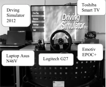
The driving simulation test was conducted at the Laboratorium of Information Management in Department of Informatics, Institut Teknologi Sepuluh Nopember using a laptop Asus N46V with the driving simulator 2012 software, Emotiv EPOC+ as the recording device, Logitech G27 driving simulator as the driving controller in the simulation test, and Toshiba Smart TV 42 inches as the screen car windshield. The designs are shown in the Figure 3.

The participants had to wear Emotiv EPOC+ device for 33 minutes to 1.5 hours as the duration for the driving simulation and the device placements.

Figure 3 The Participant Test Designs

Laptop Asus N46V

Emotiv EPOC+ Logitech G27

Toshiba Smart TV Drving

ISSN: 1992-8645 www.jatit.org E-ISSN: 1817-3195

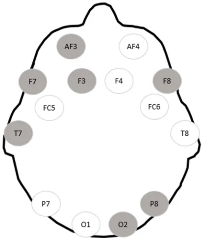
350 The Emotiv EPOC+ device channels that used in this paper are 14 channels, the location of the channels are shown in the Figure 4.

Figure 4 The Location of The Emotiv EPOC+ Channels

2.3 Participant Requirements

The participants are recruited from the Department of Informatics with the number participants is 30 people. Every participant had undergone screening criteria as follows: adults (≥ 18 years with mean age 20,4 years), experienced with riding a vehicle (minimum experience was 3 months), understand and remembered the questionnaire, and the steps to mention the degree of the driving fatigue state.

2.4 Test Environments and Procedures

The environment of the driving simulation are as follows:

a. The track used is a circuit. b. Max gear is second.

c. Both hands are on the steering wheel. d. The track used has minimum turns.

e. The body and head movement should be minimized.

f. No traffic light.

g. The allowed transmissions are manual/semi-automatic.

h. The participants may not talk during the driving simulation test.

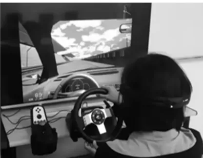
The tests will be held in 60 minutes for men and 33 minutes for women. The Figure 5 shows the example of the driving simulation test.

Figure 5 Example of The Driving Simulation Test

For every 3 minutes (it will be considered as one trial) the participants will be asked their degree of the driving fatigue state by mentioning it with their fingers (1/2/3/4/5) based on the modified Karolinska Sleepiness Scale (KSS) questionnaire. The modified KSS questionnaire is shown in the Figure 6.

Figure 6 The Modified KSS Questionnaire

If the participants feel unable to complete the required time, the participants could raised their hand and the driving simulation will be terminated.

2.5. Statistical Analysis

ISSN: 1992-8645 www.jatit.org E-ISSN: 1817-3195

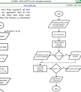
351 After the features have been acquired, all trial data in participants are appended, then do the correlation between the label data from each participant with all data trial features as illustrated in the Figure 7.

Figure 7 Get The Features of The Trial Data In All Participants

The boundary between the participants not outliers and the participant outliers is the 3 highest correlations in their channels should with the average correlation coefficient > 0,45. If the 3 highest correlations in the participant are under the boundary, then the participant data will be marked as participant outliers and would not be used as the database.

After all participants have been correlated, then find the significant channels with the frequently shown channels in 3 highest correlations from all participants. After the frequently shown channels have been acquired, then pick half of the channels with count ≥ 7 of the frequently shown in the 3 highest correlations.

The methods to find the significant channels and the participant not outliers are illustrated in the Figure 8.

Figure 8 The Illustration To Determine The Participant Outliers and To Find The Significant Channels

2.6. Feature Extraction

In the feature extraction process, the data will be divided per channel, and the FFT will be done for every channel. The TAG3 wave band mean and standard deviation will be taken as the data features. The extracted features will be placed in one dimensional array for all channels. The feature extraction process is illustrated in the

Figure 9

ISSN: 1992-8645 www.jatit.org E-ISSN: 1817-3195

352

2.7. Classification

The classification process compares between the SVM classification method and the KNN classification method in order to determine the best classification method for the driving fatigue state detection.

The classification process is used in the two processes:

a. Accuracy Test. b. Prediction.

2.7.1 Accuracy Test

The test accuracy is used to find the quality of the classification methods, since the goals are to get better results without preprocessing methods and to compare between the KNN and SVM classification method in the driving fatigue state case.

The extracted features data will be divided into testing data and training data. The training data will act as the database while the other ones will act as the target data.

The testing data is trained by the training data to determine the driving fatigue state, and the prediction results are compared with the actual label data to know the accuracy of the proposed methods.

2.7.2 Prediction

The prediction is almost as the same as the accuracy test method, the different thing is that for the feature extraction, it also do the feature extraction of the input data from the user. The classification will use the training data as the database to classify the extracted features input data.

3. RESULTS

This section shows the results of the classification method that has been proposed.

3.1 Statistical Analysis

First, do correlation between the participant data and their label from participant answers to get the good subjects and channels, then pick the ones with r > 0,45. The results of the statistical analysis method to find the participant not outliers are shown in the Table 1.

Table 1 Participant Not Outlier (The Ones With The Gray Colors)

Participant 3 Channels highest r

3 Values Channels highest r

1 2 3 1 2 3

1 7 9 8 0,46 0,38 0,33

2 2 13 6 0,66 0,63 0,59

3 13 8 2 0,20 0,17 0,13

4 10 8 11 0,72 0,63 0,56

5 3 14 12 0,53 0,49 0,31

6 11 8 13 0,45 0,40 0,39

7 9 14 3 0,51 0,45 0,44

8 1 4 3 0,47 0,44 0,30

9 12 5 13 0,52 0,43 0,43

10 1 12 9 0,57 0,56 0,56

11 3 1 7 0,90 0,77 0,73

12 12 8 3 0,33 0,29 0,29

13 2 9 8 0,44 0,39 0,38

14 5 14 10 0,46 0,32 0,28

15 9 13 2 0,52 0,50 0,45

16 5 9 8 0,81 0,80 0,75

17 1 2 12 0,64 0,62 0,56

18 3 5 2 0,82 0,80 0,70

19 9 6 2 0,33 0,22 0,19

20 5 1 13 0,78 0,69 0,38

21 7 3 9 0,54 0,52 0,51

22 3 14 5 0,57 0,52 0,49

23 7 3 8 0,84 0,81 0,76

24 9 4 5 0,77 0,50 0,50

25 1 2 3 NaN NaN NaN

26 9 12 8 0,64 0,63 0,59

27 4 5 10 0,71 0,65 0,63

28 9 7 11 0,59 0,50 0,47

29 1 2 3 NaN NaN NaN

30 13 11 4 0,73 0,66 0,48

ISSN: 1992-8645 www.jatit.org E-ISSN: 1817-3195

353

Table 2 The Significant Channels That Are Shown in The 3 Highest Correlations Channels With Counts ≥ 7 (The Ones With Gray Colors).

Channel Nama Channel

Count

1 AF3 7

2 F7 9

3 F3 11

4 FC5 4

5 T7 8

6 P7 2

7 O1 5

8 O2 9

9 P8 11

10 T8 3

11 FC6 4

12 F4 6

13 F8 7

14 AF4 4

When the outlier channels and participants have been determined, group the data without the outlier participants into their respective classes.

Figure 10 shows the significant channels that will be used as the features that will represent the data.

Figure 10 The Significant Channels That Will Be Used For The Classification Process (The Ones With The gray Colors).

Figure 11 shows the results of the FFT process on the channel 2 that will taken their theta, alpha, beta, and gamma wave features (mean and standard deviation) to represent the data for the classification processes.

Figure 11 The FFT Results From The Channel 2 (AF3) That Will be Used to Get The Features of The Data: (a) Theta, (b) Alpha, (c) beta, and (d) gamma

3.2 Accuracy Test

The accuracy test uses fold=10 and 10 loops, where each loops will randomize the testing data and the training data using cross validation. The results of the accuracy test contains mean accuracy, maximum accuracy, minimum accuracy, standard (std) accuracy, true positive (TP) score, true negative (TN) score, false positive (FP) score, and false negative (FN).

The user interface application of the accuracy test process is shown in the Figure 12.

ISSN: 1992-8645 www.jatit.org E-ISSN: 1817-3195

354 x

Figure 12 The User Interface of The Accuracy Test Application to Show the Accuracy Results of The Proposed Methods

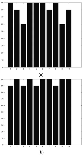
The accuracy test results using the proposed methods are shown in the Figure 13.

Figure 13 The Accuracy Test Results Using: (a) SVM Classification Method and (b) KNN Classification Method

The detail of the accuracy test results is shown in the Table 3.

Table 3 The Detail of The Accuracy Test Results Using (a) SVM Classification Method and (b) KNN Classification Method

The Accuracy Test Results using The SVM Classification Method

No Specification Percentage (%)

1 Mean Accuracy SVM 81

2 Maximum Accuracy SVM

90

3 Minimum Accuracy SVM

60

4 Standard Deviation Accuracy SVM

11,97

5 True Positive SVM 43

6 True Negative SVM 38

7 False Positive SVM 4

8 False Negative SVM 15

The Accuracy Test Results using The KNN Classification Method

No Specification Percentage (%)

1 Mean Accuracy SVM 96

2 Maximum Accuracy

SVM 100

3 Minimum Accuracy

SVM 90

4 Standard Deviation

Accuracy SVM 5,16

5 True Positive SVM 45

6 True Negative SVM 51

7 False Positive SVM 2

8 False Negative SVM 2

3.3 Prediction

The user interface application of the prediction process is shown in the Figure 14.

(b) (a)

ISSN: 1992-8645 www.jatit.org E-ISSN: 1817-3195

355

Figure 14 The User Interface Application of The Prediction Process

The prediction process gives the result whether the driver is in the fatigue/sleepy state or in the alert/fit state. The prediction result is shown in the Figure 15.

Figure 15 The Prediction Results of The Input Data: (a) In The Alert/Fit State, or (b) In The Fatigue/Sleepy State

4. DISCUSSION

Based on the statistical analysis results in the Table 1, it shows that the participant not outliers are consist of 15 out of 30 participants. The reason why the other participants are not selected is because some of the participants were not fully concentrating to the driving simulation, i.e. move the body or head and the intensity of the noise in the test room. These factors resulted in the inequality of the concentration that cause the low correlation between the participant EEG data and the label. The other reason is because the participants sometimes confused in expressing their driving fatigue state, that could lead to the low of correlation results.

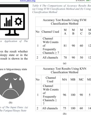
The comparisons of accuracy results between with the selected channels (count of frequently shown channels ≥ 7) and classification methods are shown in the Table 4with MA as Mean Accuracy, MB as Maximum Accuracy, MC as Minimum Accuracy, and MD as Standard Deviation.

Table 4 The Comparisons of Accuracy Results Between (a) Using SVM Classification Method and (b) Using KNN Classification Method

Accuracy Test Results Using SVM Classification Method

No Channel Used M A

M B

M C

M D

1

Channel With Counts of

Frequently Channels ≥ 7

81 90 60 12

2 All channels 70 90 50 12

Accuracy Test Results Using KNN Classification Method

No Channel

Used MA MB MC MD

1

Channel With Counts of

Frequently Channels ≥ 7

96 100 90 5

2 All channels 75 100 60 14

In the Figure 10 and Table 2 are shown the significant channels based on the frequently shown channels in the 3 highest correlation channels. The reasons of finding the significant channels are because of the time consumption and the influential channels. The time consumption that needed to process the complex data is limited, so with choosing only the influential channels could reduce the time cost and remove the unwanted noise. Hence, the accuracy results get higher and the processing time goes faster as shown in the Table 4.

ISSN: 1992-8645 www.jatit.org E-ISSN: 1817-3195

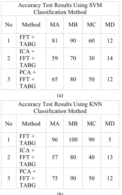
356 The comparisons of accuracy results with/without the denoising method is shown in the Table 5 with Theta, Alpha, Beta, and Gamma waves as TABG.

Table 5 The Comparisons of Accuracy Results With/Without The Denoising Method (ICA/PCA) and (a) SVM Classification Method or (b) KNN Classification Method

Accuracy Test Results Using SVM Classification Method

No Method MA MB MC MD

1 FFT +

TABG 81 90 60 12

2

ICA + FFT + TABG

59 70 30 14

3

PCA + FFT + TABG

65 80 50 12

Accuracy Test Results Using KNN Classification Method

No Method MA MB MC MD

1 FFT +

TABG 96 100 90 5

2

ICA + FFT + TABG

57 80 40 13

3

PCA + FFT + TABG

75 90 50 12

Table 5 shows that the accuracy test results without the denoising methods give better accuracy results than with the denoising methods with the average accuracy of 81% using the SVM classification method and 96% using the.KNN classification method.

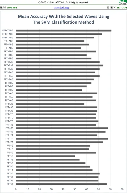
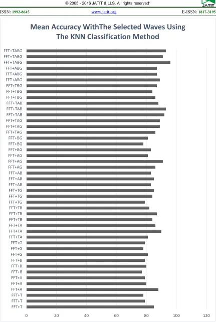
Figure 16 and Figure 17 show that the accuracy test results using TABG waves give the best accuracy result.

5. CONCLUSIONS

The conclusions of the proposed methods are as follows:

a. The classification results using KNN classification method gives betterof better

mean accuracy than using SVM classification method with a ratio of the mean accuracy of 96% and 81%.

b. Using all the waves (TABG) resulted in better accuracy with average accuracy of 96% (SVM) and 81% (KNN) compared to using one/part of the band wave.

c. The accuracy results using the selected channels (channels 1, 2, 3, 5, 8, 9, and 13) give better accuracy than using all of the channels.

d. The proposed methods without the denoising methods give better accuracy results than with the denoising methods.

ACKNOWLEDGEMENTS

This research is supported by Institut Teknologi Sepuluh Nopember and the Ministry of Research, Technology and Higher Education of Indonesia.

REFERENCES:

[1] V. Saudale, "Berita Satu," 26 October 2015.

[Online]. Available:

http://www.beritasatu.com/gaya- hidup/317264-menkes-1000-remaja-di- indonesia-meninggal-akibat-kecelakaan-lalu-lintas.html.

[2] J. P. Sasongko, "Lebih dari 2000 Kecelakaan Terjadi di Jakarta Dalam 5 Bulan," CNN Indonesia, DKI Jakarta, 2015.

[3] "Driver Fatigue and Road Accidents," The Royal Society for the Prevention of Accidents, June 2011. [Online]. Available:

http://www.rospa.com/road-safety/advice/drivers/fatigue/road-accidents/. [Accessed 20 12 2015].

[4] "Facts," National Sleep Foundation, 2015.

[Online]. Available:

http://drowsydriving.org/about/. [Accessed 20 12 2015].

[5] L. W. Ko, W. K. Lai, W. G. Liang, C. H. Chuang, S. W. Lu, Y. C. Lu, T. Y. Hsiung, H. H. Wu and C. T. Lin, "Single Channel Wireless EEG Device for Real-Time", IJCNN,

2015, pp. 1-5.

[6] F. Wang, J. Lin, W. Wang and H. Wang, "EEG-based mental fatigue assessment during driving by using sample entropy and rhythm energy", Cyber Technology in Automation, Control and Intelligent Systems, 2015, pp. (b)

ISSN: 1992-8645 www.jatit.org E-ISSN: 1817-3195

357 1906 - 1911.

[7] R. Ahmed, K. Emon and M. Hossain, "Robust driver fatigue recognition using image processing", Informatics, Electronics & Vision (ICIEV), 2014, pp. 1-6.

[8] M. A. Li, "An EEG-based method for detecting drowsy driving state", Fuzzy Systems and Knowledge Discovery (FSKD),

2010,pp. 2164 - 2167.

[9] B. C. Chang, J. E. Lim, H. J. Kim and B. H. Seo, "A study of classification of the level of sleepiness for the drowsy driving prevention",

SICE, 2007, pp. 3084 - 3089.

[10] Wikipedia, "Electroencephalography", Wikipedia, 5 February 2016. [Online]. Available:

https://en.wikipedia.org/wiki/Electroencephal ography. [Accessed 9 February 2016]. [11] I. A. Akbar, T. Igasaki, N. Murayama and a.

Z. Hu, "Drowsiness Assessment Using Electroencephalogram in Driving Simulator Environment".

[12] C. Papadelis, C. Kourtidou-Papadeli, P. Bamidis and I. Chouvarda, "Indicators of Sleepiness in an ambulatory EEG study of night driving", Engineering in Medicine and Biology Society (EMBS), 2006,pp. 6201 - 6204.

[13] B. Jap, S. Lal, P. Fischer and E. Bekiaris, "Using Spectral Analysis to Extract

Frequency Components from

Electroencephalography: Application for Fatigue Countermeasure in Train Drivers",

Wireless Broadband and Ultra Wideband Communications (AusWireless), 2007, p. 13. [14] N. Gurudath and H. B. Riley, "Drowsy

Driving Detection by EEG Analysis Using Wavelet Transform and K-means Clustering",

Procedia Computer Science, Vol. 34, 2014, pp. 400-409.

[15] C. Lin, R. C. Wu, S. F. Liang and W. H. Chao, "EEG-Based Drowsiness Estimation for Safety Driving Using Independent Component Analysis", IEEE TRANSACTIONS ON CIRCUITS AND SYSTEMS, Vol. 52, No. 12, 2005, pp. 2726 - 2738.

[16] R. Sarno, B. A. Sanjoyo, I. Mukhlash and H. M. Astuti, "Petri Net Model of ERP Business Process Variation for Small and Medium Enterprises", Journal of Theoretical and Applied Information Technology, vol. 51, no.

1, 2013, pp. 31-38.

[17] R. Sarno, C. A. Djeni, I. Mukhlash and D. Sunaryono, "Developing a Workflow Management System for Enterprise Resource Planning", Journal of Theoretical and Applied Information Technology, vol. 72, no. 3, 2015, pp. 412-421.

[18] R. Sarno, R. D. Dewandono, T. Ahmad, M. F. Naufal and F. Sinaga, "Hybrid Association Rule Learning and Process Mining for Fraud Detection", IAENG International Journal of Computer Science, vol. 42, no. 2, 2015,pp. 59-72,.

[19] A. H. Basori, R. Sarno and S. Widyanto, "The Development of 3D Multiplayer Mobile Racing Games Based On 3D Photo Satellite Map", Proceedings of the IASTED International Conference on Wireless and Optical Communications, 2008, pp. 1-5. [20] R. Sarno, P. Sari, H. Ginardi dan D.

ISSN: 1992-8645 www.jatit.org E-ISSN: 1817-3195

358

Figure 16 Mean Accuracy With The Selected Waves Using The SVM Classification Method

0 10 20 30 40 50 60 70 80 90

FFT+T FFT+T FFT+T FFT+A FFT+A FFT+A FFT+B FFT+B FFT+B FFT+G FFT+G FFT+G FFT+TA FFT+TA FFT+TA FFT+TB FFT+TB FFT+TB FFT+TG FFT+TG FFT+TG FFT+AB FFT+AB FFT+AB FFT+AG FFT+AG FFT+AG FFT+BG FFT+BG FFT+BG FFT+TAG FFT+TAG FFT+TAG FFT+TAB FFT+TAB FFT+TAB FFT+TBG FFT+TBG FFT+TBG FFT+ABG FFT+ABG FFT+ABG FFT+TABG FFT+TABG FFT+TABG

ISSN: 1992-8645 www.jatit.org E-ISSN: 1817-3195

359

Figure 17 Mean Accuracy WithThe Selected Waves Using The KNN Classification Method

0 20 40 60 80 100 120

FFT+T FFT+T FFT+T FFT+A FFT+A FFT+A FFT+B FFT+B FFT+B FFT+G FFT+G FFT+G FFT+TA FFT+TA FFT+TA FFT+TB FFT+TB FFT+TB FFT+TG FFT+TG FFT+TG FFT+AB FFT+AB FFT+AB FFT+AG FFT+AG FFT+AG FFT+BG FFT+BG FFT+BG FFT+TAG FFT+TAG FFT+TAG FFT+TAB FFT+TAB FFT+TAB FFT+TBG FFT+TBG FFT+TBG FFT+ABG FFT+ABG FFT+ABG FFT+TABG FFT+TABG FFT+TABG