A Multi-stage Learning Method with the Selection of Training Data for the Layered Neural Networks

A Multi-stage Learning Method with the Selection of

Training Data for the Layered Neural Networks

Isao Taguchi

, Yasuo Sugai

*

Faculty of International Studies, Keiai University, Japan **

Faculty of Engineering, Chiba University, Japan

Abstract- This paper proposes an efficient learning method for the layered neural networks based on the selection of training data. The multilayer neural network is widely used due to its simple structure. When learning objects are complicated, the problems, such as unsuccessful learning or a significant time required in learning, remain unsolved. The aims of this paper are to suggest solutions of these problems and to reduce the total learning time.

Focusing on the input data during the learning stage, we undertook an experiment to identify the data that makes large errors and interferes with the learning process. Our method devides the learning process into several stages.

Computational experiments suggest that the proposed method has the capability of higher learning performance and needs less learning time compared with the conventional method. And, compares the QPROP and RPROP methods by computation experiments using function approximation problems as an example and demonstrates the efficacy of integrating the proposed method with either method.

Index Terms- Multi-layer Neural Network, Data Selection, Multi-stage Learning, Integrating the Proposed Method with Either Method

I. INTRODUCTION

ajority of neural network research focuses on complicated networks such as pulsed neural networks [1]. However, in reality, multilayer neural networks (NNs) that are composed of sigmoid units using back propagation (BP) are widely used because of their simple structures.

In our previous paper [2], we proposed a comprehensive learning method that features the categorization of training data based on the ease of learning prior to initiating a learning session. Multi-stage learning based on the dynamic adjustment of the learning rate in response to error size and input characteristics to the output layer unit (effectively utilizing amplitude diminishing conditions and desired value acquisition conditions) was applied in complex learning cases that require the use of large quantities of learning data.

Proactive use of the oscillation characteristic of BP through the proposed method [2] is expected be effective when integrated with the Quick-Prop method (QPROP method) [4], an extension of BP, or when integrated with the elastic/resilient BP method (RPROP method) [5]. The QPROP method makes adjustments that are as large as possible to the learning rate while also adding an inertia term to the weight coefficient variation to suppress

oscillation. To avoid oscillation due to sudden changes in the weight coefficient, it also applies a maximum variation limit. Generally, three coefficients—the learning coefficient, the maximum variation, and the weight renewal suppression coefficient—are required. Furthermore, the elastic BP method [5] confirms the weight renewal code and suppresses oscillation to accelerate learning. Normally, it is a method that learns by adjusting five parameters such as the learning coefficient in response to current conditions. In both methods, learning occurs with acceleration parameters while oscillation is suppressed.

In this study, we report the effects of the integration of the proposed method with QPROP and RPROP on error and learning time.

The remainder of this paper is composed as follows. Section 2 discusses the QPROP and RPROP methods. Section 3 compares the QPROP and RPROP methods by computation experiments using function approximation problems as an example and demonstrates the efficacy of integrating the proposed method with either method. Section 4 summarizes our findings.

II. EFFICIENT LEARNING METHODS

Paper [2] discusses the dynamic adjustment of the learning coefficient in response to error, input characteristics to the output layer unit, the selection of learning data, and effective learning methods based on these properties. Here we will briefly discuss the QPROP and RPROP methods.

2.1. QPROP method and RPROP method

The QPROP method [5] is one of the BP methods where learning speed is enhanced while learning coefficients are made as large as possible and inertial terms are added to the amount of change of weight coefficients. The inertial terms are where the weights are updated by considering the previous amount of updated weight as well as the present amount of updated weight. That is, when the amount of corrected weight at the time k is obtained, the formula will be as follows by considering the amount of corrected weight of (k-1):

(k)= (k)+ (k-1) (1)

But,

(k)=

+λ (k) (2)

and the weight is updated with the Formula (k=1,2,…) where the subscript i is a middle layer unit i, and the subscript j means the output layer unit j. The mark λis a suppressing coefficient of

updating weights. Let the learning coefficient be = when either of the conditions of be or

(k) is met and let the learning coefficient

be =0 when none of the conditions is met. For the inertial

term , calculate ̃ =

and let = when either

of the conditions of ̃ > or ̃ < 0 is

met and let = ̃ when the answer does not meet any of the conditions.

The RPROP method [6] is where suppressed-vibration learning is carried out by adjusting five parameters in accordance with conditions, while the previous amount of updated weight should be memorized to suppress vibrations and a sign of the previous amount of updated weight and that of the current amount of updated weight are taken into consideration. Let

*

and the amount of updated weight varies

depending on signs of m. Basically, weights are updated based on the three formulas indicated below. The formulas feature that

is set so that the updated amount will not be so large

and is set so that the updated amount will not be so small.

m>0

(k )=min( (k -1)* , =－sign(

)* (k ) (3)

m<0

(k )=max( (k -1)* ,

m=0

=－sign(

)* (k ) (5)

Table 1 Learning Functions

III. COMPUTATIONAL EXPERIMENTS USING FUNCTION APPROXIMATION PROBLEMS AS EXAMPLES

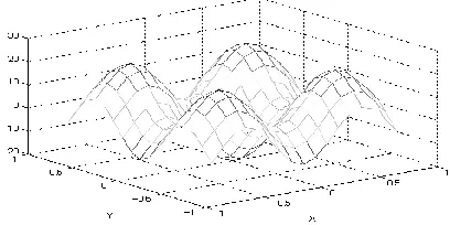
To demonstrate the efficacy of the multistage learning method proposed in this study, we perform computational experiments using function approximation problems as an example. These problems have been chosen, because the difficulty of learning can be configured with the selection of different functions, and experiments of unlearned data can be verified easily. A number of useful functions are the well-known Rastrigin and Ridge functions for optimization problems. These are given in Table (1).

3.1. Training Data

Table (1)(a) is shown in Figure 1. In Figure 1, adjacent training data are shown joined by a solid line. The region to learn in Table (1)(a) is given as −0.8 x, y 0.8 for the Rastrigin function. The training data sets the x, y direction stride as 0.1 and partitions the region into a 17 × 17 (289 point) grid given as training data set D.

Table (1)(b) gives the region to learn as −6.0 x, y 6.0 for the Ridge function. The training data sets the x, y direction stride as 1.2 and partitions the region into an 11 × 11 (121 point) grid given as the training data set D.

3.2. Training Data Selection

Here we discuss the method used to select the training data in Table (1)(a) for many experiments due to the difficulty of learning. The selection of the training data in table(1)(a)can be substituted with values obtained by the partial differentiation of functions fx(x, y) or fy(x, y) in both x and y directions.

Figure 1. An example of characteristics of the target function

Next, we divide the training data into three steps (s = 3) and perform multistage learning. uses approximately 30%

(a) Rastrigin Function

f(x,y)=x2-10cos(2 x) +y2-10cos (2 y) -0.8 x 0.8，-0.8 y 0.8 ) -20.0 f(x,y) 20.5

(b)Ridge Function

f(x,y)= 2x2+2xy+y2

of all training data. and (selected using the values of fx(x, y) or fy(x, y) are important, because they grasp the outline of the function. The final number of data included in was 31.1% (90 pieces). Within this data, 24 pieces fulfilled |f(x, y) 0.90, 34 fulfilled |fx(x, y) 0.3, and 34 fulfilled |fy(x, y) 60.3. Two pieces were repeated; thus, the total was 90 pieces.

Table 2 : The method of Learning(Ridge Function)

In step 2, the final number of data included in was 58.1% (168 pieces). Within this data, 52 pieces fulfilled |f(x, y)| 0.80, 68 pieces fulfilled |fx(x, y) 60.1, and 68 pieces fulfilled |fy(x, y)| 60.1. Twenty pieces were repeated; thus, the total was 168 pieces.

In in step 3, all data was used. Thus, 31.1% of all data was used in step 1, 58.1% of all data was used in step 2, and 100% of all data was used in the final step. Table (2) shows this information for Table (1)(b). As a feature of the Ridge function shown in Table (1)(b), because |f(xi, yi)| becomes larger when the values of |fx(xi, yi)| or |fy(xi, yi)| increase, the training data was selected on the basis of the values of |fx(xi, yi)| and |fy(xi, yi)|.

3.3.Experiment Settings for Methods Used in Comparison

To verify the efficacy of the proposed method, the results of computational experiments were compared with those of existing methods. The NN used for the proposed method, existing method, QPROP method, RPROP method, and learning method, with the integrated proposed method, is a three-layer feed-forward network using sigmoid elements. This is composed of two

input-layer elements, nine middle-input-layer elements, and one output-input-layer element. The number of middle-layer elements was determined by preliminary experiments. All weight coefficients were renewed once per epoch in each method. The learning count for the proposed method was 2333 epochs for step one, 2333 epochs for step two, and 2334 epochs for step three for a total of 7000 epochs. The two existing methods used all training data for 7000 epochs of learning. Computations were performed on a 3.0GHz Pentium 4 PC with 2GB RAM operating on Windows XP. The basic learning coefficient for the proposed method and existing methods was η = 0.8 (standard). To evaluate the learning results, the RMSE values for the training data and average weight sets for four initial weight coefficient values were used. Weight coefficient initial values were set randomly in a range from −0.01 to 0.01.

By a number of preliminary experiments, the QPROP parameters were set as follows. The weight variation suppression coefficient λ = 0.005, maximum change amount μ = 0.95, learning coefficient η1 = 0.80, and by adjusting the direction of weights, the learning coefficient η2 = 0.12. For RPROP experiments conducted, the following parameters were used: Δmax = 5.0, Δmin = 0.0025, η+ = 0.97, η−= 0.89, η0 = 0.61.

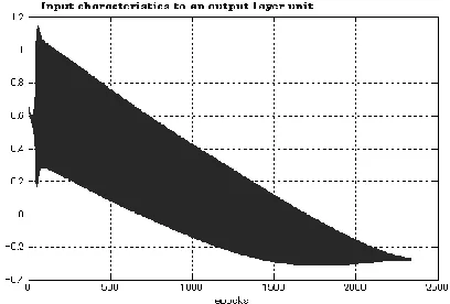
Figure 2. Input characteristics for the +QPROP methods in the output unit(Ridge function, )

Figure 3. Input characteristics for the +RPROP methods in the output unit(Ridge function, )

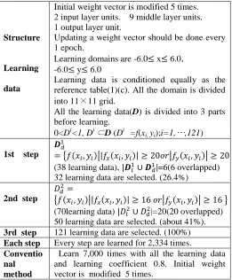
Structure

Learning

data

Initial weight vector is modified 5 times. 2 input layer units. 9 middle layer units. 1 output layer unit.

Updating a weight vector should be done every 1 epoch.

Learning domains are -6.0 x 6.0， -6.0 y 6.0

Learning data is conditioned equally as the reference table(1)(c). All the domain is divided into 11×11 grid.

All the learning data(D) is divided into 3 parts before learning.

0<Di<1, Di ⊂D (Di =f(xi, yi);i=1,…,121)

1st step

{ | | | }

(38 learning data), |=6(6 overlapped) 32 learning data are selected. (26.4%)

2nd step _{{ | | | }}

(70learning data) |=20(20 overlapped) 50 learning data are selected. (about 41%).

3rd step 121 learning data are selected. (100%)

Each step Every step are learned for 2,334 times.

Conventio nal method

3.4. Computational Experiment Results

Table 3 displays the learning results using the proposed method and the QPROP and RPROP methods independently, as well as the results of using the QPROP and RPROP methods with the proposed method integrated. The values shown in Table 3 is the averages for five experiments conducted with five different initial weight values selected randomly.

As shown in Table 3, integrating the proposed method with the RPROP or QPROP method improved the RMSE (mean) value and decreased the learning time when learning with the Ridge function (Figures 2 and 3).

As shown in Table 4, when the proposed method is applied to the Rastrigin function shown in Table (1)(a), all RMSE values are below 0.1 when the learning coefficient (the standard when using the proposed method) is between 0.9 and 0.2. When the learning coefficient decreases to 0.1 or 0.05, the RMSE values increase above 0.1, but the useful range of the learning coefficient value is extremely wide.

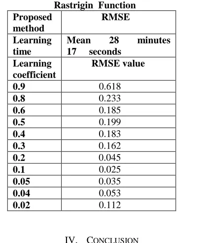
Conversely, as shown in Table 5, learning was carried out while changing the learning coefficient in the range from 0.9 to 0.02 for the two existing methods as well. From 0.9 to 0.3, no learning occurred with the RMSE values above 0.1. From 0.2 to 0.04, the RMSE value decreased below 0.1(Mean learning time = 28 minutes 17 seconds). Conversely, when reduced to 0.02, the RMSE value increased above 0.1.

When learning using existing methods with a constant learning coefficient of 0.04, oscillation occurs in the final 2334 repetitions, and the RMSE value is 0.053. These results are shown in Table 5. The input characteristics to the output layer unit are shown in Figure 4.

3.5. Considering the Experimental Results

Here we consider the performance and calculation time of learning by integrating the proposed method with the QPROP and RPROP methods on an NN and discuss the necessity of oscillation based on the computational experiment results. Integrating the Proposed Method into QPROP and RPROP Methods

Figure 4. Input characteristics for the traditional methods in the output layer.

Table 3: RMSE for Proposed Methods and Traditional Methods in Learning of the Ridge Function

As shown in Table 3, by integrating the proposed method with the QPROP and RPROP methods, the RMSE average when learning with the Ridge function reduced in comparison with that before integration. In independent learning before integration, average error values for the RPROP method, proposed method, and QPROP method were 0.050, 0.107, and 0.172, respectively. However, by integrating the proposed method into the RPROP method, error reduced to 0.036. Integration with the QPROP method reduced the error from 0.172 to 0.058. When the QPROP and RPROP methods were used independently, the input characteristics to the output element unit showed almost no oscillation, but integrating the proposed method added a small amount of oscillation.

RMSE

Mean Maximum Minimum

value value

Proposed method

0.107 0.235 0.038

Learning time

Mean 6 minutes 59 seconds

Proposed method+QP ROP

0.058 0.113 0.024

Learning time

Mean 7 minutes 10 seconds

QPROP method

0.172 0.241 0.108

Learning time

Mean 10 minutes 24 seconds

RPROP method

0.050 0.080 0.023

Learning time

Mean 13 minutes 52 seconds

Proposed method+ RPROP method

0.038 0.051 0.030

Learning time

Table 4: RMSE for Proposed Methods in Learning of the Rastrigin Function

Proposed method

RMSE

Learning time

Mean 15 minutes 56 seconds

Learning coefficient

RMSE value

0.9 0.050

0.8 0.126

0.7 0.037

0.6 0.027

0.5 0.026

0.4 0.039

0.3 0.081

0.2 0.096

0.1 0.138

0.05 0.135

Table 5: RMSE for Traditional Methods in Learning of the Rastrigin Function

Proposed method

RMSE

Learning time

Mean 28 minutes

17 seconds

Learning coefficient

RMSE value

0.9 0.618

0.8 0.233

0.6 0.185

0.5 0.199

0.4 0.183

0.3 0.162

0.2 0.045

0.1 0.025

0.05 0.035

0.04 0.053

0.02 0.112

IV. CONCLUSION

This study discussed a comprehensive learning method for neural networks that categorized training data based on the ease of learning before learning, performed multistage learning based on those categories, and dynamically adjusted the learning coefficient in response to error size. Experiments were conducted by integrating the method with QPROP and RPROP methods. As a result, the RMSE value decreased, and the learning time improved.

In future studies, we will actively use oscillation characteristics, extend the proposed method to evaluate effects on pattern recognition problems, and investigate further decreases in error.

References

[1] Makoto Motoki，Seiichi Koakutsu，Hironori Hirata:``A Supervised Learning Rule Adjusting Input-Output Pulse Timing for Pulsed Neural Network'', The transactions of the Institute of Electronics, Information and Communication Engineers, Vol.J89-D- {II}, No.12, pp.726-734 (2006) [2] Isao Taguchi and Yasuo Sugai :``An Efficient Learning

Method for the Layered Neural Networks Based on the Selection of Training Data and Input Characteristics of an Output Layer Unit'', The Trans. of The Institute of Electrical engineers of Japan, Vol.129-C, No.4, pp.1208-1213, (2009) [3] Isao Taguchi and Yasuo Sugai :``An Input Characteristic of

Output Layer Units in the Layered Neural Networks and Its Application to an Efficient Learning'', Proc. of the Electronics, Information and Systems Conference, Electronics, Information and systems Society, IEE. of Japan, pp.931-934 (2004)

[4] Falleman, D.E.,:``An Empirical Study of Learning Speed in Back-Propagation Network'', Technical Report CMU-CS-88-162, Carnegie-Mellon University, Computer Sceinece Dept., (1988)

[5] M. Riedmiller and H. Braun,:``A DirectbAdaptive Method for Faster Backpropagation Learning: The \rm{RPROP} Algorithm'', Proc. ICNN, San Fransisco, (1993)

[6] Nobuyuki Matsui and kenichi Ishimi:``A Multilayered Neural Network Including Neurons with fluctuated Threshold'', The Trans. of The Institute of Electrical Engineers of Japan, Vol.114-C, No.11, pp.1208-1213 (1994)

[7] Ting Wang and Yasuo Sugai:``A Wavelet Neural Network for the Approximation of Nonlinear multivariable Functions'', The Trans. of The Institute of Electrical engineers of Japan, Vol.120-C, No.2, pp.185-193 (2000) [8] Yasuo Sugai，Hiroshi Horibe, and Tarou Kawase:``Forecast

of Daily Maximum Electric Load by Neural Networks Using the Standard Electric Load'', The Trans. of The Institute of Electrical engineers of Japan, Vol.117-B, No.6, pp.872-879 (1997)

[9] Souichi Umehara, teru Yamazaki, and Yasuo Sugai:``A Precipitation Estimation System Based on Support Vector Machine and Neural Network'', The transactions of the Institute of Electronics, Information and Communication Engineers, Vol.J86-D-\rm{II}, No.7, pp.1090-1098 (2003) [10] Ting Wang and Yassuo Sugai:``A Wavelet Neural

Network for the Approximation of Nonlinear Multivariable Functions'', Proc.of IEEE International Conference on System, Man, and Cybernetics, \rm{III}, pp.378-383 (1999)

[11] L.Ｋ.Jones:``Constructive Approximations for Neural Networks by Sigmoidal Functions'', Proc. IEEE, Vol.78, No.10, pp.(1990)

[12] B.Irie and S.Miyake:``Capabilities of Three Layered Perceptrons'', Proc.ICNN, Vol.1, pp.641-648 (1988) [13] K. Funahashi:``On the Approximate Realization of

Continuous Mapping by Neural Networks'', Vol.2, No.3, pp.183-192 (1989)

Determination of Viscosity in Water-TiO2 Nanofluid'', Advances in Mechanical Engineering, Article ID 742680, Volume 2012 , , 10 pages, (2012)

[15] Neng-Sheng Pai, Her-Terng Yau, Tzu-Hsiang Hung, and Chin-Pao Hung: ``Application of CMAC Neural Network to Solar Energy Heliostat Field Fault Diagnosis'', International Journal of Photoenergy, Article ID 938162, 8 pages Volume 2013, 8 pages, (2013)

AUTHORS

Isao Taguchi received the D.Eng. Course of

urban environmental systems, graduate school of engineering, Chiba University, Japan, in 2011.

I am a professor, course of Faculty of international studies, Keiai university, in 2005. My research area are the neural networks, information science, information education, and their applications. I am a member of IEEJ. [email protected]

Yasuo Sugai received the D.Eng. degree from