An Alternating Direction Nonmonotone Approximate Newton Algorithm for Inverse Problems

(1)

http://www.scirp.org/journal/jamp ISSN Online: 2327-4379

ISSN Print: 2327-4352

An Alternating Direction Nonmonotone

Approximate Newton Algorithm for Inverse

Problems

Zhuhan Zhang, Zhensheng Yu, Xinyue Gan

University of Shanghai for Science and Technology, Shanghai, China

Abstract

In this paper, an alternating direction nonmonotone approximate Newton algorithm (ADNAN) based on nonmonotone line search is developed for solving inverse prob-lems. It is shown that ADNAN converges to a solution of the inverse problems and numerical results provide the effectiveness of the proposed algorithm.

Keywords

Nonmonotone Line Search, Alternating Direction Method, Bound-Constraints, Newton Method

1. Introduction

We consider inverse problems that can be expressed in the form

( )

2

1 min

2 Ax b− +φ Bx , (1)

where A∈Rm n× ,B∈Rm n× , :φ Rm→ −∞ ∞

(

,

)

is convex, and m

b∈R . The emphasis of

our work is on problems where A and B have a specific structure. It can be applied to many applications, especially in machine learning [1][2], image reconstruction [3][4] or model reduction [5]. We assume that the functions in (1) are strictly convex, so both problems has an unique solution *

x .

In Hong-Chao Zhang’s paper [6], he uses the Alternating Direction Approximate Newton method (ADAN) based on Alternating Direction Method (ADMM) which ori-ginaly in [7] to solve (1). He employs the BB approximation to increase the iterations. In many applications, the optimization problems in ADMM are either easily resolvable, since ADMM iterations can be performed at a low computational cost. Besides,

com-How to cite this paper: Zhang, Z.H., Yu, Z.S. and Gan, X.Y. (2016) An Alternating Direction Nonmonotone Approximate New-ton Algorithm for Inverse Problems. Journal of Applied Mathematics and Physics, 4, 2069- 2078.

http://dx.doi.org/10.4236/jamp.2016.411206

Received: October 28, 2016 Accepted: November 27, 2016 Published: November 30, 2016

http://creativecommons.org/licenses/by/4.0/

(2)

bine different Newton-based methods with ADMM have become a trend, see [6][8][9], since those methods may achieve the high convergent speed.

In alternating direction nonmonotone approximate Newton (ADNAN) algorithm developed in this paper, we adopt the nonmonotone line search to replace the tradi-tional Armijo line search in ADAN, because the nonmonotone schemes can improve the likelihood of finding a global optimum and improve convergence speed in cases where a monotone scheme is forced to creep along the bottom of a narrow curved val-ley in [10].

In the latter context, the first subproblem is to solve the unconstrained minimization problems with Alternating Direction Nonmonotone Approximate Newton algorithm. The purpose is to accelerate the speed of convergence, and then to project or the scale the unconstrained minimizer into the box

{

w∈Rm:l≤ ≤w u

}

, The second

subprob-lem is a bound-constrained optimization probsubprob-lem.

The rest of the paper is organized as follows. In Section 2, we give a review of the al-ternating direction approximate Newton method. In Section 3, we introduce the new algorithm ADNAN. In Section 4, we introduce the gradient-based algorithm of the second subproblem. A preliminary convergence analysis for ADNAN and gradient- based algorithm (GRAD) is given in Section 5. Numerical results presented in Section 6 explain the effectiveness of ADNAN and GRAD.

2. Review of Alternating Direction Approximate Newton

Algorithm

In this section, we briefly review the well-known Alternating Direction Approximate Newton (ADAN) method which has been studied in the areas of convex programming and image reconstruction see [4][6] and references therein.

We introduce a new variable w to obtain the split formulation of (1):

( )

2 ,

1

min s.t. , ,

2

n m

x w Ax b− +φ w w=Bx x∈R w∈R (2)

The augmented Lagrangian function associated with (2) is

(

)

1 2

( ) (

)

2

, ,

2 2

L x wλ = Ax b− +φ w +λ Bx−w +β Bx−w (3)

where β>0 is the penalty parameter, b∈Rm is a Lagrangian multiplier associated

with the constraint w=Bx. In ADMM, each iteration minimizes over x holding w

fixed, minimizes over w holding x fixed, and updates an estimate for the multiplier b. More specifically, if λk_{is the current approximation to the multiplier, then ADMM}

[10][11] applied to the split formulation (3) is given by the iteration:

(

)

1

arg min , ,

k k k

x

x + = L x w λ (4)

(

)

1 _{arg min} 1_{, ,}

k k k

w

w+ = L x + wλ (5)

(

)

1

k k k k

w Bx

λ + ₌λ ₊β ₋ ₍₆₎

(3)

( )

1

arg min

k

x

x+ = f x

( )

₂ 2

1

2 2

k k

f x = Ax b− +β Bx−w +β λ− (7)

For any Hermitian matrix N N

Q∈R × , we define x_Q2 = x Qx, , if Q is a positive

de-finite matrix, then •_Q is a norm. The proximal version of (4) is

( )

1

arg min

k

x

x+ = f x

( )

₂ 2

1

2 2

k k k

Q

f x = Ax−b +β Bx−w +β λ− + −x x (8)

In ADAN, the choice _Q₌δ_I₋_{A A}T will cancel the _Ax2 term in this iteration

while 2

Bx is retained. We replace δ by δ_k, where δ_kI is a Barzilai-Borwein (BB)

[8][12] approximation to T

A A. We can observe the fast convergence of BB

approxi-mation in the experiments of Raydan and Svaiter [13]. Moreover, δk is strictly smaller

than the largest eigenvalue of T

A A, and Q=δ_kI−A AT is indefinite, so the new

convergence analysis is needed. As a result, the updated version for x given in (4) can be expressed as follows:

( )

(

)

1

1 T T

arg min

k k

k x

x + = f x =x − A A+βB B − ∇f (9)

(

)

(

)

T T 1

: k k k k

k

f A Ax b βB Bx w β λ−

∇ = − + − + (10)

Here,

( )

1

. − is the generalized inverse, T T

A A+βB B is the Hessian of the objective

f , and ∇f is the gradient of f at xk, gk = ∇f . The formula for

1

k

x + in (2) is

exactly the same formula that we would have gotten if we performed a single iteration of Newton’s method on the equation ∇f x

( )

=0 with starting guess xk. We employ

the BB approximation T

k

A A≈δ I, [14] where

(

) (

)

{

}

(

)

2 1 1 min 2 1 min 2 1

arg min :

max ,

k k k k

k

k k

A x x x x

A x x

x x

δ δ δ δ

δ − − − − = − − − ≥  ₋    = _ _ −    

and δmin>0 is a positive lower bound for δk. Hence, the Hessian is approximated by

T kI B B

δ +β . Since a Fourier transform can be inverted in O N

(

logN

)

flops. The

in-version of T

kI B B

δ + can be accomplished relatively quickly. After replacing T

A A

by δkI, the iteration becomes

1

k k

k

x + =x +d where d_k = −

(

δ_kI+βB BT

)

−1∇f_k

Note that by substituting T

k

Q=δ I−A A in (2) and solving for the minimizer, we

would get exactly the same formula for the minimizer as that given in (5). When the search direction is determined suitable step size αk along this direction should be found to determine the next iterative point such as k 1 k

k k

x+ =x +α d .

The inner product between dk and the objective gradient at xk is

(

2 2

)

,

k k k k k

f d δ d β Bd

(4)

It follows that dk is a descent direction. Since f is a quadratic, the Taylor expan-sion of

( )

k 1

f x+ around k

x is as follows:

( ) ( )

2

1 1 1 1

,

2

k k k k k k

k _H

f x+ = f x + ∇f x + −x + x+ −x

where _H ₌_{A A}T ₊β_{B B}T

Algorithm 1. Nonmonotone Line search

In this section, we adopt a nonmonotone line search method [9]. The step size αk is chosen in an ordinary Armijo line search which could not admit the more faster speed in unconstrained problems [12]. In contrast, nonmonotone schemes can not only im-prove the likelihood of finding a global optimum but also imim-prove convergence speed.

Initialization: Choose starting guess x0 , and parameters 0≤ηmin≤ηmax ≤1, 0<m<σ< <1 ρ, and u>0. Set C0 = f x

( )

0 , Q0 =1, and k=0.

Convergence test: If f x

( )

k sufficiently small, then stop.

line search update: set xk+1=xk+αkd dk, k =0,where αk satisfies either the (nonmonotone) Wolfe conditions:

(

_k _k _k

)

_k _k

( )

_k _k,

f x +α d ≤C +mα∇f x d (11)

(

k k k

)

k

( )

k k

f x α d d σ f x d

∇ + ≥ ∇ (12)

or the (nonmonotone) Armijo conditions: hk

k

α =αρ , where α >k 0 is the trial step, and hk is the largest integer such that (11) holds and αk ≤µ.

Cost update: Choose ηk∈

[

ηmin,ηmax

]

, and update

( )

(

)

1 1, 1 1 1

k k k k k k k k k

Q₊ =η Q + C₊ = η Q C + f x₊ Q₊ (13)

Observe that Ck+1 is a convex combination of Ck and f x

(

k+1

)

. Since C0 = f x

( )

0

it follows that Ck is a convex combination of the function values f x

( )

0 ,,f x

( )

k . The

choice of ηk controls the degree of nonmonotonicity. If η =k 0 for each k, then the line search is the usual monotone Wolfe or Armijo line search. If η =k 1 for each k,

then Ck =Ak where

( )

0 1

, 1

k

k i i i

i

A f f f x

k =

= =

+

∑

, is the average function value. The

scheme with Ck = Ak was proposed by Yu-Hong Dai [15]. As ηk approaches 0, the line search closely approximates the usual monotone line search, and as ηk ap-proaches 1, the scheme becomes more nonmonotone, treating all the previous function values with equal weight when we compute the average cost value Ck.

Lemma 2.1 If f x

( )

_k d_k ≤0 for each k, then for the iterates generated by the

nonmonotone line search algorithm, we have fk ≤Ck≤Ak for each k. Moreover, if

( )

_k _k 0 f x d <

 and f x

( )

is bounded from below, then there exists αk satisfying

either the Wolfe or Armijo conditions of the line search update.

3. Alternating Direction Nonmonotone Approximate Newton

Algorithm

(5)

is an unconstrained minimization problem with ADNAN, then to project or the scale the unconstrained minimizer into the box

( )

2 1 min , 2 n

l w u≤ ≤ Ax−b +φ Bx x∈R (14)

the iteration is as follows:

(

)

1

arg min , ,

k k k

x

x + = L x w λ (15)

(

)

1 _{arg min} 1_{, ,}

k k k

l w u

w+ L x+ wλ

≤ ≤

= ₍₁₆₎

(

)

1

k k _wk _Bxk

λ + ₌λ ₊β ₋

(17) Later we give the existence and uniqueness result for (1).

The solution k

w to (5) has the closed-form means

(

)

arg min , ,

k

k k k k

l w u

w L x w b P Bx λ

β

≤ ≤

 

= = _ − _

 

with P being the projection map onto the box

[ ]

l u, .

Algorithm 2. Alternating Direction Nonmonotone Approximate Newton algo-rithm.

Parameter: 0.5< < <γ 1 τ ρ, >0, 0<δmin<δ0, Initialize k=1.

Step 1: If f x

( )

k sufficiently small, then set

1

1 , 0,

k k k

k k

x+ =x d = δ =δ ₋ , and

branch to Step 4.

(

)

2

1 min 2 1 max , k k k k k

A x x

x x δ δ − −  ₋    =   −    

,

(

_T

)

1

.

k k k

d = − δ I+βB B − ∇f

Step 2: If δ αk k >δ α δk−1 k, k >max

{

δmin,δk−1

}

then δmin=τδmin.

Step 3: If αk accomplish the Wolfe conditions, then αk:=ταmax.

Step 4: Update x which generated from Algorithm 1.

Step 5: 1

. k

k k

w P Bx λ

β

+ ₌  ₋ 

 

 

Step 6: 1

(

1 1

)

.

k k k k

b + =b +β Bx + −w+

Step 7: If a stopping criterion is satisfied, terminate the algorithm, Otherwise k = k + 1 and go to Step 1.

Lemma 3.1: we show some criteria that are only satisfied a finite number of times, so

min

δ converge to positive limits. An upper bound for δmin is the following:

Uniformly in k, we have δmin,k ≤δk ≤max

{

δ τ, A

}

where δmin,k is the value of

min

δ at the start of iteration k and δ δ= min,1 is the starting δmin in ADAN.

Lemma 3.2: If Adk =Bdk =0, then k

x minimizes f x

( )

_k .

4. Algorithm 3: Gradient-Based Algorithm (GRAD)

(6)

( )

2 1 min , 2 n

l x u≤ ≤ Ax b− +φ Bx w∈R (18)

And the iteration is similar with (4) (5) (6) as follows:

(

)

1

arg min , ,

k k k

l x u

x + L x w λ

≤ ≤

= (19)

(

)

1 1

arg min , ,

k k k

w

w + = L x + wλ (20)

(

)

1

k k k k

w Bx

λ + ₌λ ₊β ₋ ₍₂₁₎

Compute the solution k

x from (19), k 1

(

k 1 k

)

x =B− λ +P w−

Compute the solution k

w from (20),

(

A AT +B B wT

)

k =A bT +βwk−1+λk

Set k 1 k

(

k k

)

w Bx

λ + ₌λ ₊β ₋

5. Convergence Analysis

In this section, we show the convergence of proposed algorithms. Obviously, the proofs of the two algorithms are almost the same, and we only prove the convergence of algo-rithm 2.

Lemma 3.1: Let L be the function in (3). The vector

(

* *

)

[ ]

, n ,

x w ∈R × l u solves (2)

if and only if there exists * n

R

λ ∈ _{such that}

(

* * *

)

, ,

x w λ solves

(

* *

) (

* * *

) (

*

)

(

)

[ ]

, , , , , , , , , n , n.

L x w λ ≤L x w λ ≤L x wλ ∀ x wλ ∈R × l u ×R

Lemma 3.2: Let L be the function in (3),

(

* * *

)

, ,

x w λ be a saddle-point of L, Then

the sequence

(

k, k

)

x w satisfies

(

) (

* *

)

lim k, k ,

k→∞ x w = x w .

Theorem 3.1: Let

(

x wk, k

)

be the sequence of iterates produced by the algorithm 2.

then *

lim k k→∞x =x ,

*

lim k

k→∞w =w and

(

)

* *

,

x w is the optimal point for problem (14)

Proof From Lemma 3.1, 3.2, we obtain that

1

0, l

lim wk+ −wk = im wk−xk =0 (22)

Since we have a unique minimizer in

[ ]

l u, , so we have lim *

k k

x x

→∞ = , Then, (22)

gives *

lim k

k→∞w =w which completes the proof.

6. Numerical Experiments

6.1. Parameter Settings

In Algorithm 2, the parameters β, the penalty in the augmented Lagrangian (3), are

common to these two algorithms, ADAN and ADNAN. Besides β _{has a vital impact}

on convergence speed. We choose 4

10

β ₌ − _{based on the results from W. Hager}_[6]_.

The choice τ =1.2 is a compromise between speed and stability, δmin =0.001 is large

enough to ensure invertibility.

(7)

objec-tive in (1), we ran them for 100,000 iterations. The optimal objecobjec-tive values for the three data sets were

0.1275 0.2456 0.9627

Ψ = Ψ = Ψ =

In addition, we timed how long it took ADNAN to reduce the objective error to within 1% of the optimal objective value. The algorithms are coded in MATLAB, ver-sion 2011b, and run on a Dell verver-sion 4510U with a 2.8 GHz Intel i7 processor.

In Algorithm 3, a 256-by-256 gray-scale image was considered, which is compared to the experiment by J. Zhang [8]. The dimensions of the inverse problems are m = n = 65536 and the constraints are l= −∞ and u=

(

255,, 255

)

T. The experiments on

image deblurring problems show that GRAD algorithm is also effective in terms of quality of the image resolution.

6.2. Experiments Results

This section compares the performance of the ADNAN to ADAN. The main difference

between the ADNAN algorithm and the ADAN algorithm is the computation of k 1

x + .

In ADAN k 1 k

k k

x+ =x +α d where α_k is the step size. In ADNAN, x generated from

Algorithm 1, if the convergence condition in ADAN is satisfied, then the update

1

k k

x + =x +α d could be performed. Here δ_k is the same choice for them. Hence,

there seems to be a significant benefit from using a value for δk smaller than the larg-est eigenvalue of T

A A.

The initial guess for 1

x , w1 and λ1 was zero for two algorithms. Figures 1-3

[image:7.595.195.553.539.689.2]

show the objective values and objective error as a function of CPU time. Moreover, we give the comparison of objective values and objective error versus CPU time/s for dif-ferent

Ψ

conditions. It is observed that ADNAN is slightly stable than ADAN al-though ADNAN and ADAN are competitive. The ADNAN not only could get more smaller objective error but also get more fast convergence speed (see Figure 3). In ad-dition, ADNAN objective value could get more smaller after a few iterations than ADAN. As a whole, the effect of ADNAN is superior to ADAN.

(8)

Figure 2. Ψ =0.2456.

[image:8.595.192.552.63.397.2]

Figure 3. Ψ =0.9627.

On the other hand, the experiment results about Algorithm 3 are as follows:

Original image blurry image deblurred image

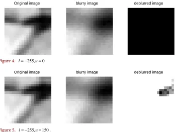
Figure 4. l= −255,u=0.

[image:8.595.196.547.440.703.2]

(9)

Figure 6. l= −255,u=200.

[image:9.595.191.556.69.352.2]

Figure 7. l= −255,u=255.

7. Conclusions

According to the Figures 1-3, we can conclude that the nonmonotone line search could accelerate the convergence speed, furthermore ADNAN could get the objective values more stable and fast during the iterations when compared to ADAN.

On the other hand, the validness of GRAD is verified. Experiments results on image deblurring problems in Figures 4-7 show that difference constraints on x can also get effective deblurred images.

Acknowledgements

This work is supported by Innovation Program of Shanghai Municipal Education Commission (No. 14YZ094).

References

[1] Amit, Y. (2007) Uncovering Shared Structures in Multiclass Classification. Machine

Learn-ing, Twenty-fourth International Conference, 227, 17-24.

https://doi.org/10.1145/1273496.1273499

[2] Argyriou, A., Evgeniou, T. and Pontil, M. (2007) Multi-Task Feature Learning. Advances in

Neural Information Processing Systems, 19, 41-48.

[3] Chambolle, A. (2004) An Algorithm for Total Variation Minimization and Applications.

Journal of Mathematical Imaging and Vision, 20, 89-97.

[4] Chambolle, A. (2011) A First-Order Primal-Dual Algorithm for Convex Problems with Ap-plications to Imaging. Journal of Mathematical Imaging and Vision, 40, 120-145.

(10)

Ap-proximation with Application to System Identification. SIAM Journal on Matrix Analysis

and Applications, 31, 1235-1256.

[6] Hager, W. and Zhang, H.-C. (2015) An Alternating Direction Approximate Newton Algo-rithm for Ill-Conditioned Inverse Problems with Application to Parallel MRI. Journal of the

Operational Research Society of China, 3, 139-162.

[7] Gabay, D. and Mercier, B. (1976) A Dual Algorithm for the Solution of Nonlinear Varia-tional Problems via Finite Element Approximations. Computers & mathematics with

ap-plications, 2, 17-40.

[8] Zhang, J.J. (2013) Solving Regularized Linear Least-Squares Problems by the Alternating Direction Method with Applications to Image Restoration. Electronic Transactions on

Numerical Analysis, 40, 356-372.

[9] Zhang, H.C. and Hager, W. (2004) A Nonmonotone Line Search Technique and Its Appli-cation to Unconstrained Optimization. Society for Industrial and Applied Mathematics, 14, 1043-1056.

[10] Grippo, L., Lampariello, F. and Lucidi, S. (1986) A Nonmonotone Line Search Technique for Newton’s Method. SIAM Journal on Mathematical Analysis, 23, 717-716.

[11] Eckstein, J. and Bertsekas, D. (1992) On the Douglas-Rachford Splitting Method and the Proximal Point Algorithm for Maximal Monotone Operators. Mathematical Programming, 55, 293-318. https://doi.org/10.1007/BF01581204

[12] Barzilai, J. and Borwein, J. (1988) Two Point Step Size Gradient Methods. IMA Journal of

Numerical Analysis, 8, 141-148. https://doi.org/10.1093/imanum/8.1.141

[13] Raydan, M. and Svaiter, B.F. (2002) Relaxed Steepest Descent and Cauchy-Barzilai-Borwein Method. Computational Optimization and Applications, 21, 155-167.

https://doi.org/10.1023/A:1013708715892

[14] Block, K.T., Uecker, M. and Frahm J. (2007) Undersampled Radial MRI with Multiple Coils: Iterative Image Reconstruction Using a Total Variation Constraint. Magnetic

Re-sonance in Medicine, 57, 1086-1098. https://doi.org/10.1002/mrm.21236

[15] Dai, Y.H. (2002) On the Nonmonotone Line Search. Journal of Control Theory and

Appli-cation, 112, 315-330.

[16] Grippo, L., Lampariello, F. and Lucidi, S. (1989) A Truncated Newton Method with Non-monotone Line Search for Unconstrained Optimization. Journal of Optimization Theory

(11)

Submit or recommend next manuscript to SCIRP and we will provide best service for you:

Accepting pre-submission inquiries through Email, Facebook, LinkedIn, Twitter, etc. A wide selection of journals (inclusive of 9 subjects, more than 200 journals)

Providing 24-hour high-quality service User-friendly online submission system Fair and swift peer-review system

Efficient typesetting and proofreading procedure

Display of the result of downloads and visits, as well as the number of cited articles Maximum dissemination of your research work