Munich Personal RePEc Archive
Large time-varying parameter VARs
Koop, Gary and Korobilis, Dimitris
University of Strathclyde, University of Glasgow
28 February 2012
Online at
https://mpra.ub.uni-muenchen.de/38591/
Large Time-Varying Parameter VARs
Gary Koop
University of Strathclyde
Dimitris Korobilis
University of Glasgow
Abstract
In this paper we develop methods for estimation and forecasting in large
time-varying parameter vector autoregressive models (TVP-VARs). To overcome
computa-tional constraints with likelihood-based estimation of large systems, we rely on Kalman
filter estimation with forgetting factors. We also draw on ideas from the dynamic model
averaging literature and extend the TVP-VAR so that its dimension can change over
time. A final extension lies in the development of a new method for estimating, in
a time-varying manner, the parameter(s) of the shrinkage priors commonly-used with
large VARs. These extensions are operationalized through the use of forgetting
fac-tor methods and are, thus, computationally simple. An empirical application involving
forecasting inflation, real output, and interest rates demonstrates the feasibility and
usefulness of our approach.
Keywords: Bayesian VAR; forecasting; time-varying coefficients; state-space model
JEL Classification: C11, C52, E27, E37
Acknowledgements:The authors are Fellows of the Rimini Centre for Economic
Analy-sis. We would like to thank the Economic and Social Research Council for financial support
under Grant RES-062-23-2646.
1
Introduction
Many recent papers (see, among many others, Banbura, Giannone and Reichlin, 2010;
Car-riero, Clark and Marcellino, 2011; CarCar-riero, Kapetanios and Marcellino, 2009; Giannone,
Lenza, Momferatou and Onorante, 2010; Koop, 2011) have found large VARs, which have
dozens or even hundreds of dependent variables, to forecast well. In this literature, the
researcher typically works with a single large VAR and assumes it is homoskedastic and its
coefficients are constant over time. In contrast to the large VAR literature, with smaller VARs
there has been much interest in extending traditional (constant coefficient, homoskedastic)
VARs in two directions. First, researchers often find it empirically necessary to allow for
parameter change. That is, it is common to work with time-varying parameter VARs
(TVP-VARs) where the VAR coefficients evolve over time and multivariate stochastic volatility is
present (see, among many others, Cogley and Sargent, 2005, Cogley, Morozov and Sargent,
2005, Primiceri, 2005 and Koop, Leon-Gonzalez and Strachan, 2009). Second, there also
may be a need for model change: to allow for switches between different restricted TVP
models so as to mitigate over-parametrization worries which can arise with parameter-rich
unrestricted TVP-VARs (e.g. Chan, Koop, Leon-Gonzalez and Strachan, 2012). The question
arises as to whether these two sorts of extensions can be done with large TVP-VARs. This
paper attempts to address this question.
Unfortunately, existing TVP-VAR methods used with small dimensional models cannot
easily be scaled up to handle large TVP-VARs with heteroskedastic errors. The main reason
this is so is computation. With constant coefficient VARs, variants of the Minnesota prior
are typically used. With this prior, the posterior and predictive densities have analytical
forms and MCMC methods are not required. With TVP-VARs, MCMC methods are required
to do exact Bayesian inference. Even the small (trivariate) TVP-VAR recursive forecasting
exercises of D’Agostino, Gambetti and Giannone (2011) and Korobilis (2012) were hugely
computationally demanding. Recursive forecasting with large TVP-VARs is typically
A first contribution of this paper is to develop approximate estimation methods for large
TVP-VARs which do not involve the use of MCMC methods and are computationally feasible.
To do this, we use forgetting factors. Forgetting factors (also known as discount factors),
which have long been used with state space models (see, e.g., Raftery, Karny and Ettler,
2010, and the discussion and citations therein), do not require the use of MCMC methods
and have been found to have desirable properties in many contexts (e.g. Dangl and Halling,
2012). Most authors simply set the forgetting factors to a constant, but we develop methods
for estimating forgetting factors in a time-varying way following an approach outlined in
Park, Jun and Kim (1991). This allows for the degree of variation of the VAR coefficients to
be estimated from the data (without the need for MCMC).
A second contribution of this paper is to add to the expanding literature on estimating
the prior hyperparameter(s) which control shrinkage in large Bayesian VARs (see, e.g.,
Giannone, Lenza and Primiceri, 2012). Our approach differs from the existing literature
in treating different priors (i.e. different values for the shrinkage parameter) as defining
different models and estimating dynamic posterior model probabilities to select the optimal
value of the shrinkage parameter at each point in time. We develop a simple recursive
updating scheme for the time-varying shrinkage parameter which is computationally simple
to implement.
A third contribution of this paper is to develop econometric methods for doing model
selection using a model space involving the large TVP-VAR and various restricted versions of
it. We define small (trivariate), medium (seven variable) and large (25 variable) TVP-VARs
and develop methods for time-varying model selection over this set of models. Interest
centers on forecasting the variables in the small VAR, and selection of the best
TVP-VAR dimension each time period is done using the predictive densities for these variables
(which are common to all the models). To be precise, the algorithm selects between small,
medium and large TVP-VARs based on past predictive likelihoods for the set of variables
the researcher is interested in forecasting. A potentially important advantage is that this
might select the large TVP-VAR as the forecasting model at some points in time, but at other
points it might switch to a small or medium TVP-VAR, etc. Such model switching cannot be
done in conventional approaches and has been found to be useful in univariate regression
applications (e.g. Koop and Korobilis, 2011). Its incorporation has the potential to be useful
in improving the forecast performance of TVP-VARs of different dimensions and to provide
information on which model forecasts best (and when it does so).
These methods are used in an empirical application involving a standard large US
quar-terly macroeconomic data set, with a focus on forecasting inflation, real output and interest
rates. Our empirical results are encouraging and demonstrate the feasibility and usefulness
of our approach. Relative to conventional VAR and TVP-VAR methods, our results highlight
the importance of allowing for the dimension of the TVP–VAR to change over time and
allowing for stochastic volatility in the errors.
2
Large TVP-VARs
2.1 Overview
In this section we describe our approach to estimating a single TVP-VAR using forgetting
factors. We write the TVP-VAR as:
yt=Zt t+"t,
and
t+1= t+ut; (1)
time series variables and
Zt= 0 B B B B B B B @
zt0 0 0
0 z0t . .. ...
..
. . .. ... 0
0 0 z0t 1 C C C C C C C A ;
where Zt is M k. zt is a vector containing an intercept and p lags of each of the M variables. Thus,k=M(1 +pM).
Once the researcher has selected a specification for t and Qt; a prior for the initial conditions (i.e. 0and possibly 0andQ0) and a prior for any remaining parameters of the
model, then Bayesian statistical inference can proceed in a straightforward fashion (see, for
instance, Koop and Korobilis, 2009, for a textbook-level treatment) using MCMC methods.
The basic idea underlying these methods is that standard methods for drawing from state
space models (i.e. involving the Kalman filter) can be used for drawing t for t = 1; ::; T
(conditional on t, Qt and the remaining model parameters). Then t for t = 1; ::; T (conditional on t; Qt and the remaining model parameters) can be drawn. Then Qt for t= 1; ::; T (conditional on t; tand the remaining model parameters) can be drawn. Then any remaining parameters are drawn (conditional on t; Qtand t).
This algorithm works well with small TVP-VARs, but can be computationally very
de-manding in larger VARs due to the fact that it is a posterior simulation algorithm. Typically,
tens of thousands of draws must be taken in order to ensure proper convergence of the
algorithm. And, in the context of a recursive forecasting exercise, the posterior simulation
algorithm must be run repeatedly on an expanding window of data. Even with constant
coefficient large VARs, Koop (2011) found the computational burden to be huge when
pos-terior simulation algorithms were used in the context of a recursive forecasting exercise.
With large TVP-VARs, the computational hurdle can simply be insurmountable.
In the next sub-section, we show how approximations using forgetting factors can greatly
reduce the computational burden by allowing the researcher to avoid the use of expensive
done, analytical formulæ exist for obtaining the posterior of t, and the one-step ahead
predictive density of the TVP-VAR model.
2.2 Estimation of TVP-VARs Using Forgetting Factors
Forgetting factor approaches were commonly used in the past, when computing power was
limited, to estimate state space models such as the TVP-VAR. See, for instance, Fagin (1964),
Jazwinsky (1970) or West and Harrison (1997) for a discussion of forgetting factors in state
space models and, in the context of the TVP-VAR, see Doan, Litterman and Sims (1984).
Dangl and Halling (2012) is a more recent application which also uses a forgetting factor
approach. Here we outline the key aspects of forgetting factor methods.
Let ys = (y1; ::; ys)0 denote observations through time s. Bayesian inference for t in-volves the Kalman filter, formulæ for which can be found in many textbook sources and will
not be repeated here (see, e.g., Fruhwirth-Schnatter, 2006, Chapter 13). But key steps in
Kalman filtering involve the result that
t 1jyt 1 N t 1jt 1; Pt 1jt 1 (2)
where formulae for t 1jt 1 andPt 1jt 1 are given in textbook sources. Kalman filtering
then proceeds using:
tjyt 1 N tjt 1; Ptjt 1 ; (3)
where
Ptjt 1 =Pt 1jt 1+Qt: (4)
Ptjt 1 = 1Pt 1jt 1 (5)
there is no longer a need to estimate or simulateQt. is called a forgetting factor which is restricted to the interval0< 1. A detailed discussion of and motivation for forgetting factor approaches is given in places such as Jazwinsky (1970) and Raftery et al (2010).
Equation (5) implies that observations j periods in the past have weight j in the filtered estimate of t. Note also that (4) and (5) imply thatQt= 1 1 Pt 1jt 1 from which it
can be seen that the constant coefficient case arises if = 1.
In papers such as Raftery et al (2010), is simply set to a number slightly less than one.
For quarterly macroeconomic data, = 0:99 implies observations five years ago receive approximately 80% as much weight as last period’s observation. This leads to a fairly
stable model where coefficient change is gradual and where has properties similar to
what Cogley and Sargent (2005) call a “business as usual” prior. These authors use exact
MCMC methods to estimate their TVP-VAR. In order to ensure that the coefficients tvary
gradually they use a tight prior on their state covariance matrixQwhich depends on a prior shrinkage coefficient which determines the prior mean. It can be shown that their choice
for prior shrinkage coefficient allows for variation in coefficients which is roughly similar to
that allowed for by = 0:99.1
A contribution of our paper is to investigate the use of forgetting factors in large
TVP-VARs. However, we go beyond most of the existing literature in two ways: we investigate
estimating (as opposed to simply setting it to a fixed value)2 and we do so in a time
varying manner. To do so, we follow a suggestion made in Park, Jun and Kim (1991) and
replace by tin (5) where
t= min+ (1 min)Lft (6)
1Note that Cogley and Sargent (2005) have a fixed state equation error covariance matrixQ, while we use a
time varying one. This does not affect the interpretation of as a shrinkage factor similar to the one they use.
2An exception to this is McCormick, Raftery, Madigan and Burd (2011) which estimates forgetting factors in
whereft= N IN T e"0t 1e"t 1 ande"t=yt tjt 1Ztis the one-step ahead prediction error produced by the Kalman filter andN IN T rounds to the nearest integer. We set min = 0:96
andL= 1:1(values calibrated to obtain a spread of values for the forgetting factor between
0:96and1:0, given our prior guess about whatE e"0te"t would tend to be).
A similar approximation is used to remove the need for a posterior simulation algorithm
for multivariate stochastic volatility in the measurement equation. In financial applications
it is common to use an Exponentially Weighted Moving Average (EWMA) filter to model
volatility dynamics (see RiskMetrics, 1996 and Brockwell and Davis, 2009, Section 1.4).
We adopt an EWMA estimator for the measurement error covariance matrix:
bt= bt 1+ (1 )e"te"0t; (7)
wheree"t = yt tjt 1Zt is produced by the Kalman filter. EWMA estimators also require the specification of the decay factor . We set = 0:96which is in the region suggested in RiskMetrics (1996). This estimator requires the choice of an initial condition, 0 for which
we use the sample covariance matrix ofy where + 1is the period in which we begin our forecast evaluation.
2.3 Model Selection Using Forgetting Factors
Our previous exposition applies to one model. Raftery et al (2010), in a TVP regression
context, develops methods for doing dynamic model averaging (DMA) and selection (DMS).
The reader is referred to Raftery et al (2010) or Koop and Korobilis (2011) for a complete
derivation and motivation of DMA. Here we provide a general description of what it does.
In subsequent sections, we use the general strategy outlined here in two ways. First, we use
DMS so as to allow for the TVP-VAR to change dimension over time. Second, we use it to
select optimal values for the VAR shrinkage parameter in a time-varying manner.
time t, given information through time t 1. Once tjt 1;j for j = 1; ::; J are obtained they can either be used to do model averaging or model selection. DMS arises if, at each
point in time, the model with the highest value for tjt 1;j is used for forecasting. Note
that tjt 1;j will vary over time and, hence, the forecasting model can switch over time.
The contribution of Raftery et al (2010) is to develop a fast recursive algorithm using a
forgetting factor for obtaining tjt 1;j.
To do DMA or DMS we must first specify the set of models under consideration. In
papers such as Raftery et al (2010) or Koop and Korobilis (2011) the models are TVP
regressions with different sets of explanatory variables. In the present paper, our model
space is of a different nature, including TVP-VARs of differing dimensions, but the basic
algorithm still holds.
DMS is a recursive algorithm where the necessary recursions are analogous to the
pre-diction and updating equations of the Kalman filter. Given an initial condition, 0j0;j for
j= 1; ::; J, Raftery et al (2010) derive a model prediction equation using a forgetting factor :
tjt 1;j =
t 1jt 1;j PJ
l=1 t 1jt 1;l
; (8)
and a model updating equation of:
tjt;j =
tjt 1;jpj ytjyt 1 PJ
l=1 tjt 1;lpl(ytjyt 1)
; (9)
wherepj ytjyt 1 is the predictive likelihood (i.e. the predictive density for modelj eval-uated atyt). Note that this predictive density is produced by the Kalman filter and has a standard, textbook, formula (e.g. Fruhwirth-Schnatter, 2006, page 405). The predictive
likelihood is a measure of forecast performance.
We refer the reader to Raftery et al (2010) for additional details (e.g. the relationship
of this approach to the marginal likelihood), but note here that the calculation of tjt;j and
the implication of the forgetting factor approach, note that tjt 1;j(the key probability used
to select models), can be written as:
tjt 1;j / t 1
Y
i=1
pj yt ijyt i 1
i
:
Thus, model j will receive more weight at time tif it has forecast well in the recent past (where forecast performance is measured by the predictive density, pj yt ijyt i 1 ). The interpretation of “recent past” is controlled by the forgetting factor, and we have the
same exponential decay as we do for the forgetting factor . For instance, if = 0:99, forecast performance five years ago receives 80% as much weight as forecast performance
last period. If = 0:95, then forecast performance five years ago receives only about 35% as much weight. These considerations suggest that, as with (or t) we focus on values of
near one and, in our empirical section, we set = 0:99.
2.4 Model Selection Among Priors
Given that we use a forgetting factor approach which negates the need to estimate Qt and use an EWMA estimate for t, prior information is required only for 0. But this
source of prior information is likely to be important. That is, papers such as Banbura et
al (2010) are working with large VARs with many more parameters than observations and
prior information is crucial in obtaining reasonable results. With TVP-VARs this need is
even greater. Accordingly, we use a tight Minnesota prior for 0. In the case where the
time-variation in parameters is removed (i.e. when t = and t = 1 for all t), this Minnesota prior on 0 becomes a Minnesota prior in a constant coefficient VAR and, thus,
this important special case is included as part of our approach.
With large VARs and TVP-VARs it is common to use training sample priors (e.g.
Prim-iceri, 2005 and Banbura et al, 2010) to elicit hyperparameters which control the degree
of shrinkage. In training sample approaches, the same prior is used as each point in time
which allows for the estimation of the shrinkage hyperparameter in a time-varying fashion.
The algorithm we develop allows for the shrinkage hyperparameter to be updated
auto-matically (in a similar fashion to the way the Kalman filter updates coefficient estimates).
In the context of a recursive forecasting exercise, an alternative strategy for having
time-varying shrinkage would be to re-estimate the shrinkage priors at each point in time and
re-estimate the model at each point in time (such an approach is used in Giannone, Lenza
and Primiceri, 2012). This can be computationally demanding (particularly if the shrinkage
parameter is estimated at a grid of values). Our automatic updating procedure avoids this
problem and is computationally much less demanding.
For a TVP-VAR of a specific dimension, we use a Normal prior for 0 which is similar to
the Minnesota prior (see, e.g., Doan, Litterman and Sims, 1984). Our empirical section uses
a data set where all variables have been transformed to stationarity and, thus, we choose
the prior mean to beE( 0) = 0. A Minnesota prior for a VAR using untransformed levels variables would set appropriate elements ofE( 0) to 1 so as to shrink towards a random walk and this can be trivially accommodated in the approach set out below.
The Minnesota prior covariance matrix for 0 is typically assumed to be diagonal and
we follow this practice. If we letvar( 0) = V andVi denote its diagonal elements, then our prior covariance matrix is defined through:
Vi=
8 > < > :
r2 for coefficients on lagrforr= 1; ::; p
afor the intercepts
; (10)
wherepis lag length. The key hyperparameter inV is which controls the degree of shrink-age on the VAR coefficients. We will estimate from the data. Note that this differs from
the Minnesota prior in that the latter contains two shrinkage parameters (corresponding to
own lags and other lags) and these are set to fixed values. Theoretically, allowing for two
shrinkage parameters in our approach is straightforward. To simplify computation we only
have one shrinkage parameter (as does Banbura et al, 2010). Finally, we seta= 103for the
In large VARs and TVP-VARs, a large degree of shrinkage is necessary to produce
rea-sonable forecast performance. We achieve this by estimating at each point in time using
the following strategy. Define a grid of values for : (1); ::; (G). We use the following very
wide grid for : 10 10;10 5;0:001;0:005;0:01;0:05;0:1 . For a Bayesian, a model contains
the likelihood and the prior. Different values for can be thought of as defining different
priors and, thus, different models. We can use the DMS methods described in the preceding
sub-section to find the optimal value for . However, before we do this, we further augment
the model space to allow for TVP-VARs of different dimensions.
2.5 Dynamic Dimension Selection (DDS)
DMA and DMS have previously been used in time-varying regression contexts where each
model is defined by the set of included explanatory variables. In the previous sub-section,
we described how DMS can be used where the models are defined by different priors. We
can also augment the model space with models of different dimensions. In particular, we
can do DMS over three models: a small, medium and large TVP-VAR. Definitions of the
variables contained in each TVP-VAR are given in the Data Appendix.
Thus, in this paper, the model space is defined by a value for and a TVP-VAR
dimen-sionality. With seven values for and three TVP-VAR sizes, we have 21 different models.
Remember that our goal is to calculate tjt 1;j for j = 1; ::J which is the probability that model j is the forecasting model at time t, given information through time t 1. When forecasting at timet, we evaluate tjt 1;j for every j and use the value of and TVP-VAR dimension which maximizes it. The recursive algorithm given in (8) and (9) can be used
to evaluate tjt 1;i. This algorithm begins with an initial condition: 0j0;j = J1 withJ = 21, which expresses a view that all possible models are equally likely.
The predictive density for each model, pj ytjyt 1 , plays the key role in DMS. When working with TVP-VARs of different dimension,yt, will be of different dimension and, hence, predictive densities will not be comparable. To get around this problem, we use the
common to all models). In our empirical work, this means the dynamic model selection is
determined by the joint predictive likelihood for inflation, output and the interest rate.
We refer to this approach, which allows for TVP-VARs of different dimension to be
se-lected at different points in time, as dynamic dimension selection or DDS. Thus, we use
notation TVP-VAR-DDS as notation for forecasting approaches which include this aspect.
3
Empirical Results
3.1 Data
Our data set comprises 25 major quarterly US macroeconomic variables and runs from
1959:Q1 to 2010:Q2. We work with a small VAR with three variables, a medium
TVP-VAR with seven and a large TVP-TVP-VAR with 25. Following, e.g., Stock and Watson (2008)
and recommendations in Carriero, Clark and Marcellino (2011) we transform all variables
to stationarity. The choice of which variables are included in which TVP-VAR is motivated
by the choices of Banbura et al (2010). The Data Appendix provides a complete listing of
the variables, their transformation codes and which variables belong in which TVP-VAR.
We investigate the performance of our approach in forecasting CPI, real GDP and the
Fed funds rate (which we refer to as inflation, GDP and the interest rate below). These are
the variables in our small TVP-VAR. The transformation codes are such that the dependent
variables are the percentage change in inflation (the second log difference of CPI), GDP
growth (the log difference of real GDP) and the change in the interest rate (the difference
of the Fed funds rate). We also standardize all variables by subtracting off a mean and
dividing by a standard deviation. We calculate this mean and standard deviation for each
variable using data from 1959Q1 through 1974Q4 (i.e. data before our forecast evaluation
3.2 Other Modelling Choices and Models for Comparison
We use a lag length of 4 which is consistent with quarterly data. Worries about
over-parameterization with this relatively long lag length are lessened by the use of the
Min-nesota prior variance, (10), which increases shrinkage as lag length increases. All of our
re-maining modelling choices are stated above. To remind the reader of the important choices
in our TVP-VAR-DDS approach:
We have a forgetting factor which controls the degree of time-variation in the VAR
coefficients which we set to = 0:99.
We have a forgetting factor, , which controls the amount of model switching of the
prior shrinkage parameter and over TVP-VAR dimensions. Consistent with Raftery et
al (2010), we set = 0:99.
We have a decay factor which controls the volatility, . Following RiskMetrics (1996)
we set = 0:96.
We compare the performance of TVP-VAR-DDS as outlined above to many special cases.
Unless otherwise noted, these special cases are restricted versions of TVP-VAR-DDS and,
thus (where relevant) have exactly the same modelling choices, priors and select the prior
shrinkage parameter in the same way. They include:
TVP-VARs of each dimension, with no DDS being done.
Time-varying forgetting factor versions of the TVP-VARs. In this case, tis constrained
to be in the interval[0:96;1]. We label such cases = tin the tables.
VARs of each dimension, obtained by setting t= 1fort= 1; ::; T.
Homoskedastic versions of each VAR.3
3When forecastingy
tgiven information throught 1, is estimated ast11
t 1
X
i=1
b
We also present random walk forecasts (labelled RW) and forecasts from a
homoskedas-tic small VAR estimated using OLS methods (labelled Small VAR OLS).
3.3 Estimation Results
The main focus of this paper is on forecasting. Nevertheless, it is useful to briefly present
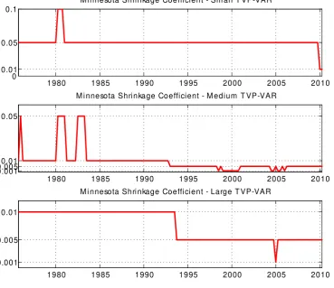
some empirical evidence on other aspects of our approach. Figure 1 plots the selected value
of , the shrinkage parameter in the Minnesota prior, at each point in time for the three
TVP-VARs of different dimension. Note that, as expected, we are finding that the necessary
degree of shrinkage increases as the dimension of the TVP-VAR increases.
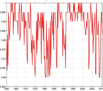
To illustrate the estimation of the time-varying forgetting factors, Figure 2 plots t
against time for the small TVP-VAR (the medium and large TVP-VARs show similar
pat-terns). Note that tdoes vary over the allowed interval of(0:96;1:0)and, hence, sometimes the VAR coefficients are changing very little, but at other times much more change is
al-lowed for. Typically, we find little change in stable times such as the 1960s and 1990s, but
more rapid change in unstable times. All periods for which tapproaches the lower bound
of 0:96 can be associated with well known events that hit the US economy (stock market crashes, oil shocks, recessions, etc.).
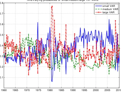
Figure 3 plots the time-varying probabilities associated with the TVP-VAR of each
di-mension. Note that, for each dimension of TVP-VAR, the optimum value for the Minnesota
prior shrinkage parameter, , is chosen and the probability plotted in Figure 3 is for this
optimum value. Remember that TVP-VAR-DDS will forecast with the TVP-VAR of dimension
with highest probability. It can be seen that there is a great deal of switching between
TVP-VARs of different dimension. In the relatively stable period from 1990 through 2007, the
small TVP-VAR is being used to forecast. For most of the remaining time DDS selects the
large TVP-VAR, although there are some exceptions to this (e.g. the medium TVP-VAR is
1980 1985 1990 1995 2000 2005 2010 0
0.01 0.05 0.1
M i nnesota Shri nkage Coefficient - Sm al l T VP-VAR
1980 1985 1990 1995 2000 2005 2010
0.001 0.0050.01 0.05
M i nnesota Shri nkage Coefficient - M edium T VP-VAR
1980 1985 1990 1995 2000 2005 2010
0.001 0.005 0.01
[image:17.595.108.478.226.545.2]M i nnesota Shri nkage Coefficient - Large T VP-VAR
1960 1965 1970 1975 1980 1985 1990 1995 2000 2005 2010 0.955
0.96 0.965 0.97 0.975 0.98 0.985 0.99 0.995 1
Estimatedλ
[image:18.595.105.467.220.538.2]t v alues - Small TVP-VAR
1960 1965 1970 1975 1980 1985 1990 1995 2000 2005 2010 0.1
0.2 0.3 0.4 0.5 0.6 0.7 0.8
Time-v ary ing probabilities of small/medium/large TVP-VARs
[image:19.595.76.496.116.442.2]small VAR medium VAR large VAR
Figure 3: Estimated Dynamic Dimension Selection probabilities of the small, medium and
large TVP-VARs.
3.4 Forecast Comparison
We present iterated forecasts for horizons of up to two years (h = 1; ::;8) with a forecast evaluation period of 1975Q1 through 2010Q2. The use of iterated forecasts does increase
the computational burden since predictive simulation is required (i.e. when h > 1 an analytical formula for the predictive density does not exist). We do predictive simulation in
the tables, does allow for coefficient change out-of-sample and simulates from the random
walk state equation (1) to produce draws of T+h. Both ways provide us with T+hand we
simulate draws ofy +h conditional on T+hto approximate the predictive density.4
The alternative would be to use direct forecasting, but recent papers such as Marcellino,
Stock and Watson (2006) tend to find that iterated forecasts are better. Direct forecasting
would also require re-estimating the model for different choices ofhand would not neces-sarily remove the need for predictive simulation since the researcher may need to simulate
T+h from (1) whenh >1.
As measures of forecast performance, we use mean squared forecast errors (MSFEs)
and predictive likelihoods. The latter are popular with many Bayesians since they evaluate
the forecast performance of the entire predictive density (as opposed to merely the point
forecast). It is natural to use the joint predictive density for our three variables of interest
(i.e. inflation, GDP and the interest rate) as an overall measure of forecast performance.
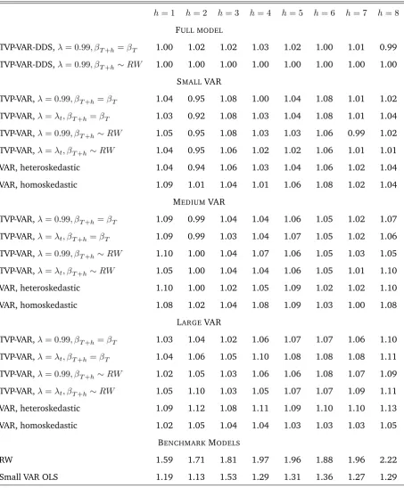
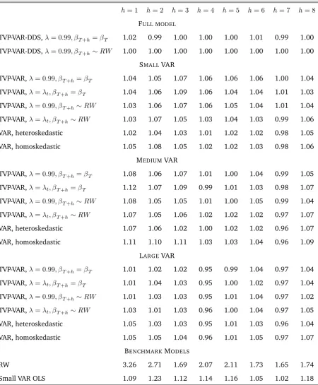
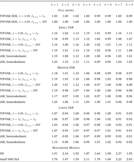
Thus, Tables 1 through 3 present MSFEs for each of our three variables of interest separately.
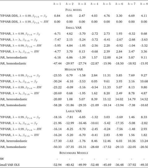
Table 4 presents sums of log predictive likelihoods using the joint predictive likelihood for
these three variables.
MSFEs are presented relative to the TVP-VAR-DDS approach which simulates T+hfrom
the random walk state equation. Tables 1 through 3 are mostly filled with numbers greater
than one, indicating TVP-VAR-DDS is forecasting better than other forecasting approaches.
This is particularly true for inflation and GDP. For the interest rate, TVP-VAR-DDS forecasts
best at several forecast horizons but there are some forecast horizons (especiallyh = 7;8) where large TVP-VARs are forecasting best. Nevertheless, overall MSFEs indicate
TVP-VAR-DDS is the best forecasting approach among the comparators we consider. Note, too, that
TVP-VAR-DDS is forecasting much better than our most simple benchmarks: random walk
forecasts and forecasts from a small VAR estimated using OLS methods.
If we consider results for TVP-VARs of a fixed dimension, it can be seen that our different
4For longer-term forecasting, this has the slight drawback that our approach is based on the model updating
implementations (i.e. different treatments of forgetting factors or methods of predictive
simulation) lead to similar MSFEs. Overall, we are finding that large TVP-VARs tend to
forecast better than small or medium ones, although there are many exceptions to this. For
instance, large TVP-VARs tend to do well when forecasting interest rates and inflation, but
when forecasting GDP the small TVP-VAR tends to do better. Such findings highlight that
there may often be uncertainty about TVP-VAR dimensionality suggesting the usefulness
of TVP-VAR-DDS. In general, though, MSFEs indicate that heteroskedastic VARs tend to
forecast about as well as TVP-VARs suggesting that, with this data set, allowing for
time-variation in VAR coefficients is less important than allowing for DDS.
With regards to predictive simulation, MSFEs suggest that simulating T+h from the
random walk state equation yields only modest forecast improvements over the simpler
strategy of assuming no change in VAR coefficients over the horizon that the forecast is
Table 1: Relative Mean Squared Forecast Errors, GDP equation
h= 1 h= 2 h= 3 h= 4 h= 5 h= 6 h= 7 h= 8
FULL MODEL
TVP-VAR-DDS, = 0:99; T+h= T 1.00 1.02 1.02 1.03 1.02 1.00 1.01 0.99
TVP-VAR-DDS, = 0:99; T+h RW 1.00 1.00 1.00 1.00 1.00 1.00 1.00 1.00
SMALLVAR
TVP-VAR, = 0:99; T+h= T 1.04 0.95 1.08 1.00 1.04 1.08 1.01 1.02
TVP-VAR, = t; T+h= T 1.03 0.92 1.08 1.03 1.04 1.08 1.01 1.04
TVP-VAR, = 0:99; T+h RW 1.05 0.95 1.08 1.03 1.03 1.06 0.99 1.02
TVP-VAR, = t; T+h RW 1.04 0.95 1.06 1.02 1.02 1.06 1.01 1.01
VAR, heteroskedastic 1.04 0.94 1.06 1.03 1.04 1.06 1.02 1.04
VAR, homoskedastic 1.09 1.01 1.04 1.01 1.06 1.08 1.02 1.04
MEDIUMVAR
TVP-VAR, = 0:99; T+h= T 1.09 0.99 1.04 1.04 1.06 1.05 1.02 1.07
TVP-VAR, = t; T+h= T 1.09 0.99 1.03 1.04 1.07 1.05 1.02 1.06
TVP-VAR, = 0:99; T+h RW 1.10 1.00 1.04 1.07 1.06 1.05 1.03 1.05
TVP-VAR, = t; T+h RW 1.05 1.00 1.04 1.04 1.06 1.05 1.01 1.10
VAR, heteroskedastic 1.10 1.00 1.02 1.05 1.09 1.02 1.02 1.10
VAR, homoskedastic 1.08 1.02 1.04 1.08 1.09 1.03 1.00 1.08
LARGEVAR
TVP-VAR, = 0:99; T+h= T 1.03 1.04 1.02 1.06 1.07 1.07 1.06 1.10
TVP-VAR, = t; T+h= T 1.04 1.06 1.05 1.10 1.08 1.08 1.08 1.11
TVP-VAR, = 0:99; T+h RW 1.02 1.05 1.03 1.06 1.06 1.08 1.07 1.09
TVP-VAR, = t; T+h RW 1.05 1.10 1.03 1.05 1.07 1.07 1.09 1.11
VAR, heteroskedastic 1.09 1.12 1.08 1.11 1.09 1.10 1.10 1.13
VAR, homoskedastic 1.02 1.05 1.04 1.04 1.03 1.03 1.03 1.05
BENCHMARKMODELS
RW 1.59 1.71 1.81 1.97 1.96 1.88 1.96 2.22
Small VAR OLS 1.19 1.13 1.53 1.29 1.31 1.36 1.27 1.29
Table 2: Relative Mean Squared Forecast Errors, Inflation equation
h= 1 h= 2 h= 3 h= 4 h= 5 h= 6 h= 7 h= 8
FULL MODEL
TVP-VAR-DDS, = 0:99; T+h= T 1.02 0.99 1.00 1.00 1.00 1.01 0.99 1.00
TVP-VAR-DDS, = 0:99; T+h RW 1.00 1.00 1.00 1.00 1.00 1.00 1.00 1.00
SMALLVAR
TVP-VAR, = 0:99; T+h= T 1.04 1.05 1.07 1.06 1.06 1.06 1.00 1.04
TVP-VAR, = t; T+h= T 1.04 1.06 1.09 1.06 1.04 1.04 1.01 1.03
TVP-VAR, = 0:99; T+h RW 1.03 1.06 1.07 1.06 1.05 1.04 1.01 1.04
TVP-VAR, = t; T+h RW 1.03 1.07 1.05 1.03 1.04 1.03 0.99 1.06
VAR, heteroskedastic 1.02 1.04 1.03 1.01 1.02 1.02 0.98 1.05
VAR, homoskedastic 1.05 1.08 1.05 1.02 1.02 1.03 0.98 1.06
MEDIUMVAR
TVP-VAR, = 0:99; T+h= T 1.08 1.06 1.07 1.01 1.00 1.04 0.99 1.05
TVP-VAR, = t; T+h= T 1.12 1.07 1.09 0.99 1.01 1.03 0.98 1.07
TVP-VAR, = 0:99; T+h RW 1.08 1.05 1.05 1.01 1.00 1.05 0.99 1.04
TVP-VAR, = t; T+h RW 1.07 1.05 1.06 1.02 1.02 1.02 0.97 1.07
VAR, heteroskedastic 1.07 1.06 1.02 1.00 1.02 1.02 0.96 1.07
VAR, homoskedastic 1.11 1.10 1.11 1.03 1.03 1.04 0.96 1.09
LARGEVAR
TVP-VAR, = 0:99; T+h= T 1.01 1.02 1.02 0.95 0.99 1.04 0.97 1.04
TVP-VAR, = t; T+h= T 1.01 1.04 1.03 0.95 1.00 1.02 0.97 1.04
TVP-VAR, = 0:99; T+h RW 1.01 1.03 1.03 0.95 1.01 1.04 0.97 1.02
TVP-VAR, = t; T+h RW 1.03 1.01 1.03 0.96 1.00 1.04 0.97 1.05
VAR, heteroskedastic 1.05 1.03 1.03 0.95 1.01 1.03 0.96 1.04
VAR, homoskedastic 1.05 1.05 1.04 0.96 1.01 1.05 0.97 1.07
BENCHMARKMODELS
RW 3.26 2.71 1.69 2.07 2.11 1.73 1.65 1.74
Small VAR OLS 1.09 1.23 1.12 1.14 1.16 1.05 1.02 1.18
Table 3: Relative Mean Squared Forecast Errors, Interest Rate equation
h= 1 h= 2 h= 3 h= 4 h= 5 h= 6 h= 7 h= 8
FULL MODEL
TVP-VAR-DDS, = 0:99; T+h= T 1.03 1.00 1.02 1.00 0.99 0.99 1.00 0.99
TVP-VAR-DDS, = 0:99; T+h RW 1.00 1.00 1.00 1.00 1.00 1.00 1.00 1.00
SMALLVAR
TVP-VAR, = 0:99; T+h= T 1.16 1.02 1.14 1.19 1.01 0.99 1.16 1.11
TVP-VAR, = t; T+h= T 1.18 0.99 1.13 1.12 1.02 0.99 1.08 1.07
TVP-VAR, = 0:99; T+h RW 1.16 1.00 1.16 1.20 1.02 1.01 1.14 1.11
TVP-VAR, = t; T+h RW 1.19 1.01 1.14 1.16 1.02 0.96 1.11 1.08
VAR, heteroskedastic 1.19 1.00 1.12 1.09 1.00 0.96 1.05 1.01
VAR, homoskedastic 1.25 1.10 1.15 1.11 0.99 0.96 1.04 1.03
MEDIUMVAR
TVP-VAR, = 0:99; T+h= T 1.18 1.01 1.10 1.06 0.98 0.99 0.98 0.97
TVP-VAR, = t; T+h= T 1.19 1.03 1.10 1.06 0.98 1.03 0.98 0.98
TVP-VAR, = 0:99; T+h RW 1.20 1.01 1.12 1.06 0.97 1.00 0.98 0.98
TVP-VAR, = t; T+h RW 1.19 0.98 1.07 1.04 1.00 1.00 0.96 0.98
VAR, heteroskedastic 1.17 0.97 1.05 1.02 0.97 1.00 0.98 0.96
VAR, homoskedastic 1.25 1.06 1.11 1.03 1.00 1.01 0.96 0.98
LARGEVAR
TVP-VAR, = 0:99; T+h= T 1.07 0.94 1.06 0.96 0.98 1.00 0.91 0.92
TVP-VAR, = t; T+h= T 1.06 0.97 1.09 0.98 1.00 1.02 0.91 0.92
TVP-VAR, = 0:99; T+h RW 1.05 0.94 1.05 0.97 0.98 1.00 0.92 0.91
TVP-VAR, = t; T+h RW 1.07 0.93 1.07 0.97 0.97 1.01 0.91 0.91
VAR, heteroskedastic 1.07 0.95 1.06 0.97 0.99 0.99 0.92 0.91
VAR, homoskedastic 1.13 0.98 1.06 0.99 1.01 1.02 0.92 0.92
BENCHMARKMODELS
RW 1.91 2.16 1.92 1.87 1.64 1.98 2.37 1.93
Small VAR OLS 1.76 1.47 1.59 2.11 1.78 1.69 2.23 2.03
Predictive likelihoods are presented in Table 4, relative to TVP-VAR-DDS. To be precise,
the numbers in Table 4 are the sum of log predictive likelihoods for a specific model minus
the sum of log predictive likelihoods for TVP-VAR-DDS. The fact that almost all of these
numbers are negative supports the main story told by the MSFEs: TVP-VAR-DDS is
forecast-ing well at most forecast horizons. Ath= 1, TVP-VAR-DDS forecasts best by a considerable margin and at other forecast horizons it beats other TVP-VAR approaches. However, there
are some important differences between predictive likelihood and MSFE results that are
worth noting.
The importance of allowing for heteroskedastic errors in getting the shape of the
pre-dictive density correct is clearly shown by the poor performance of homoskedastic models
in Table 4. In fact, the heteroskedastic VAR exhibits the best forecast performance at many
horizons. However, the dimensionality of this best forecasting model differs across
hori-zons. For instance, at h = 2 the small model forecasts best, but at h = 3 the medium model wins and ath = 4it is the large heteroskedastic VAR. This suggests, even when the researcher is using a VAR (instead of a TVP-VAR), DDS still might be a useful as a
conserva-tive forecasting device which can forecast well in a context where there is uncertainty over
Table 4: Relative Predictive Likelihoods (PLs), Total (all 3 variables)
h= 1 h= 2 h= 3 h= 4 h= 5 h= 6 h= 7 h= 8
FULL MODEL
TVP-VAR-DDS, = 0:99; T+h= T 0.84 0.91 2.47 4.03 4.76 3.30 6.69 4.11
TVP-VAR-DDS, = 0:99; T+h RW 0.00 0.00 0.00 0.00 0.00 0.00 0.00 0.00
SMALLVAR
TVP-VAR, = 0:99; T+h= T -6.71 4.62 -3.70 -2.72 2.73 1.93 -0.32 0.68
TVP-VAR, = t; T+h= T -7.47 2.15 -5.24 -3.72 -0.41 -2.67 -2.68 -3.63
TVP-VAR, = 0:99; T+h RW -5.95 4.84 -1.95 -2.56 2.20 -0.92 -1.04 -3.32
TVP-VAR, = t; T+h RW -4.77 3.70 0.13 -0.68 2.39 2.84 3.47 3.36
VAR, heteroskedastic -6.18 6.86 -1.39 1.57 12.00 6.24 5.87 9.11
VAR, homoskedastic -47.44 -29.97 -27.74 -22.87 -15.96 -18.50 -18.92 -15.93
MEDIUMVAR
TVP-VAR, = 0:99; T+h= T -23.55 0.79 -1.58 2.84 11.31 5.85 7.69 9.27
TVP-VAR, = t; T+h= T -30.24 -6.10 -3.53 0.05 9.61 3.93 3.16 10.68
TVP-VAR, = 0:99; T+h RW -23.22 -0.09 -3.16 -0.54 11.33 5.07 8.13 9.80
TVP-VAR, = t; T+h RW -20.69 0.68 -1.95 1.62 8.20 2.49 8.78 4.87
VAR, heteroskedastic -20.89 1.08 5.07 8.39 15.12 14.02 14.79 14.52
VAR, homoskedastic -58.28 -31.86 -29.35 -21.09 -10.14 -13.94 -7.38 -10.65
LARGEVAR
TVP-VAR, = 0:99; T+h= T -18.16 -7.81 -6.85 -1.32 3.03 -3.69 1.46 8.33
TVP-VAR, = t; T+h= T -21.96 -12.99 -16.46 -10.61 -5.42 -17.35 -5.08 -2.82
TVP-VAR, = 0:99; T+h RW -16.14 -8.25 -9.70 -2.45 -0.24 -7.56 -1.48 2.93
TVP-VAR, = t; T+h RW -16.24 -5.20 -6.70 -0.41 2.83 -5.90 1.56 1.82
VAR, heteroskedastic -17.30 -1.63 -1.76 8.46 12.46 6.03 10.36 13.24
VAR, homoskedastic -50.33 -37.35 -35.31 -28.60 -17.52 -29.13 -22.05 -20.50
BENCHMARKMODELS
RW - - -
-Small VAR OLS -52.94 -40.42 -49.99 -52.48 -45.69 -36.48 -37.92 -49.35
4
Conclusions
In this paper, we have developed computationally feasible methods for forecasting with
large TVP-VARs through the use of forgetting factors. We use forgetting factors in several
ways. First, they allow for simple forecasting within a single TVP-VAR model. However,
inspired by the literature on dynamic model averaging and selection (see Raftery et al,
2010), we also use forgetting factors so as to allow for fast and simple dynamic model
selection. That is, we develop methods so that the forecasting model can change at every
point in time.
DMS can be used with any type of model. We have found it useful to define our models
in terms of the priors that they use and their dimension. The former allows us to estimate
the shrinkage parameter of the Minnesota prior in a time-varying fashion using a simple
recursive updating scheme. The latter allows the TVP-VAR dimension to change over time.
In our empirical exercise, we have found our approach to offer moderate improvements in
forecast performance over other VAR or TVP-VAR approaches.
It would be simple to extend the general modelling framework presented here in several
ways. For instance, instead of using model selection methods to select prior
hyperparame-ters or TVP-VAR dimension, it would have been straightforward to use model averaging. It
would also have been possible to use DDS methods with VARs instead of TVP-VARs. Another
extension would be to use this approach for variable selection in a TVP-VAR. Suppose, for
instance, that a researcher was interested in forecasting a particular variable (e.g.
infla-tion) and had 9 potential predictors. We could define a model space which includes the
10 dimensional TVP-VAR, all 9 dimensional TVP-VARs which included inflation as one of
the variables, all 8 dimensional TVP-VARs, etc. Doing DMS using the approach outlined
over this large model space would be computationally demanding, but would allow the
researcher to select the appropriate predictors for inflation (and allow the set of predictors
to change over time). In sum, we would argue that doing DMS using forgetting factors is a
References
Banbura, M., Giannone, D. and Reichlin, L. (2010). “Large Bayesian vector auto
regres-sions,”Journal of Applied Econometrics, 25, 71-92.
Brockwell, R. and Davis, P. (2009). Time series: Theory and methods (second edition).
New York: Springer.
Carriero, A., Clark, T. and Marcellino, M. (2011). “Bayesian VARs: Specification choices
and forecast accuracy,” Federal Reserve Bank of Cleveland, working paper 11-12.
Carriero, A., Kapetanios, G. and Marcellino, M. (2009). “Forecasting exchange rates
with a large Bayesian VAR,”International Journal of Forecasting, 25, 400-417.
Chan, J., Koop, G., Leon-Gonzalez, R. and Strachan, R. (2012).“Time varying dimension
models,”Journal of Business and Economic Statistics, forthcoming.
Cogley, T., Morozov, S. and Sargent, T. (2005). “Bayesian fan charts for U.K. inflation:
Forecasting and sources of uncertainty in an evolving monetary system,” Journal of
Eco-nomic Dynamics and Control, 29, 1893-1925.
Cogley, T. and Sargent, T. (2001). “Evolving post World War II inflation dynamics,”
NBER Macroeconomics Annual, 16, 331-373.
Cogley, T. and Sargent, T. (2005). “Drifts and volatilities: Monetary policies and
out-comes in the post WWII U.S.,”Review of Economic Dynamics, 8, 262-302.
D’Agostino, A., Gambetti, L. and Giannone, D. (2009). “Macroeconomic forecasting and
structural change,”Journal of Applied Econometrics, forthcoming.
Dangl, T. and Halling, M. (2012). “Predictive regressions with time varying coefficients,”
Journal of Financial Economics,forthcoming.
Doan, T., Litterman, R. and Sims, C. (1984). “Forecasting and conditional projections
using a realistic prior distribution”,Econometric Reviews,3, 1-100.
Fagin, S. (1964). “Recursive linear regression theory, optimal filter theory, and error
analyses of optimal systems,”IEEE International Convention Record Part i, pages 216-240.
Springer.
Giannone, D., Lenza, M., Momferatou, D. and Onorante, L. (2010). “Short-term
in-flation projections: a Bayesian vector autoregressive approach,” ECARES working paper
2010-011, Universite Libre de Bruxelles.
Giannone, D., Lenza, M. and Primiceri, G. (2012). “Prior selection for vector
autore-gressions,”Centre for Economic Policy Research,working paper 8755.
Jazwinsky, A. (1970). Stochastic Processes and Filtering Theory. New York: Academic
Pres.
Koop, G. (2011). “Forecasting with medium and large Bayesian VARs,” Journal of
Ap-plied Econometrics, forthcoming.
Koop, G. and Korobilis, D. (2009). “Bayesian multivariate time series methods for
em-pirical macroeconomics,”Foundations and Trends in Econometrics, 3, 267-358.
Koop, G. and Korobilis, D. (2011). “Forecasting inflation using dynamic model
averag-ing,”International Economic Review, forthcoming.
Koop, G., Leon-Gonzalez, R. and Strachan, R. (2009). “On the evolution of the monetary
policy transmission mechanism,”Journal of Economic Dynamics and Control, 33, 997-1017.
Korobilis, D. (2012). “VAR forecasting using Bayesian variable selection”, Journal of
Applied Econometrics, forthcoming.
Marcellino, M., Stock, J. and Watson, M. (2006). “A comparison of direct and iterated
AR methods for forecasting macroeconomic series h-steps ahead,”Journal of Econometrics,
135, 499-526.
McCormick, T., Raftery, A. Madigan, D. and Burd, R. (2011). “Dynamic logistic
regres-sion and dynamic model averaging for binary classification,”Biometrics, forthcoming.
Park, D., Jun, B. and Kim, J. (1991). “Fast tracking RLS algorithm using novel variable
forgetting factor with unity zone,”Electronics Letters, 27, 2150-2151.
Primiceri, G. (2005). “Time varying structural vector autoregressions and monetary
policy,”Review of Economic Studies, 72, 821-852.
via dynamic model averaging: Application to a cold rolling mill,”Technometrics, 52, 52-66.
RiskMetrics (1996). Technical Document (Fourth Edition). Available at http://www.
riskmetrics.com/system/files/private/td4e.pdf.
Stock, J. and Watson, M. (2008). “Forecasting in dynamic factor models subject to
struc-tural instability,” inThe Methodology and Practice of Econometrics, A Festschrift in Honour of
Professor David F. Hendry, edited by J. Castle and N. Shephard, Oxford: Oxford University
Press.
West, M. and Harrison, J. (1997). Bayesian Forecasting and Dynamic Models, second
A
Data Appendix
All series were downloaded from Federal Reserve Bank of St. Louis’ FRED database and
cover the quarters 1959:Q1 to 2010:Q2. Some series in the database were observed only
on a monthly basis and quarterly values were computed by averaging the monthly values
over the quarter. All variables are transformed to be approximately stationary following
Stock and Watson (2008). In particular, if zi;t is the original untransformed series, the transformation codes are (column Tcode below): 1 - no transformation (levels),xi;t =zi;t; 2 - first difference,xi;t =zi;t zi;t 1; 3 - second difference,xi;t=zi;t zi;t 2; 4 - logarithm,
xi;t = logzi;t; 5 - first difference of logarithm, xi;t = lnzi;t lnzi;t 1; 6 - second difference
[image:31.595.163.415.354.433.2]of logarithm,xi;t= lnzi;t lnzi;t 2.
Table A1: Series used in the Small VAR withn= 3
Series ID Tcode Description
GDPC96 5 Real Gross Domestic Product
CPIAUCSL 6 Consumer Price Index: All Items
FEDFUNDS 2 Effective Federal Funds Rate
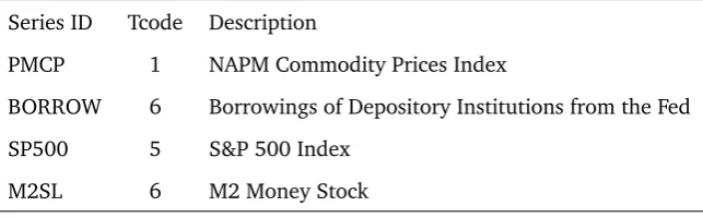
Table A2: Additional series used in the Medium VAR withn= 7
Series ID Tcode Description
PMCP 1 NAPM Commodity Prices Index
BORROW 6 Borrowings of Depository Institutions from the Fed
SP500 5 S&P 500 Index
[image:31.595.128.450.466.566.2]Table A3: Additional Series used in the Large VAR withn= 25
Series ID Tcode Description
PINCOME 6 Personal Income
PCECC96 5 Real Personal Consumption Expenditures
INDPRO 5 Industrial Production Index
UTL11 1 Capacity Utilization: Manufacturing
UNRATE 2 Civilian Unemployment Rate
HOUST 4 Housing Starts: Total: New Privately Owned Housing Units
PPIFCG 6 Producer Price Index: All Commodities
PCECTPI 5 Personal Consumption Expenditures: Chain-type Price Index
AHEMAN 6 Average Hourly Earnings: Manufacturing
M1SL 6 M1 Money Stock
OILPRICE 5 Spot Oil Price: West Texas Intermediate
GS10 2 10-Year Treasury Constant Maturity Rate
EXUSUK 5 U.S. / U.K Foreign Exchange Rate
GPDIC96 5 Real Gross Private Domestic Investment
PAYEMS 5 Total Nonfarm Payrolls: All Employees
PMI 1 ISM Manufacturing: PMI Composite Index
NAPMNOI 1 ISM Manufacturing: New Orders Index
B
Technical Appendix
B.1 Estimation and forecasting for large TVP-VAR using forgetting factors
Consider the state-space model
yt = xt t+"t (B.1)
t = t 1+ t (B.2)
where tis the unknown state vector (the VAR coefficients of the mean), and"t N(0; t). Given the initial condition 0 N(b0; P0)5and initial values 0 on t, we need to run the following Kalman recursion for periodst= 1; :::; T:
Kalman filter algorithm with forgetting factor:
Predict step
Set tjt 1= t 1jt 1
Estimate t= min+ (1 min)Lft, whereft= N IN T e"0t 1e"t 1
SetPtjt 1 = 1tPt 1jt 1
where fort= 1we use the fact that 0j0 =b0 andP0j0=P0.
Update step
Estimatee"t=yt xt tjt 1(measurement residual)
Estimatebt= bt 1+ (1 )e"te"0twhere fort= 1it simply holds that b1 = 0.
Estimate tjt= tjt 1+Ptjt 1x0t bt+xtPtjt 1x0t
1
e"t.
EstimatePtjt=Ptjt 1 Ptjt 1x0t bt+xtPtjt 1x0t
1
xtPtjt 1
5In the paper we setb
These steps are straightforward to implement, and most importantly they imply only one
run of the recursion. The most computationally expensive step is the inversion of then n
innovation covariance matrix bt+xtPtjt 1x0t . Note that xt = In 1; yt0 1; :::; y0t p 0
and the large prior covariance matrix P0 have many zeros in their structure, so sparse
matrix calculations can easily be implemented in MATLAB. An additional challenge is the
choice of the (prior) parameters min and , however these can be elicited fairly easily
following the suggestions in the paper.
The one-step ahead predictive density of the VAR is readily available from the Kalman
filter as
p yt+1jyt N xt+1 t+1jt;bt+1+xt+1Pt+1jtx0t+1
Note here the timing convention: t+1jtandPt+1jtwill be estimated from the “predict step” of the Kalman filter as tjt and 1
tPtjt, respectively, xt+1 contains lags of the dependent
variables dated yt or earlier, and bt+1 is equal bt given knowledge at time t. Hence the predictive density fort+ 1depends only on quantities we know at timetand its estimation is trivial using the analytical formula above.
For multi-step ahead forecasting we need to rely on predictive simulation (Monte Carlo).
Forecasting using predictive simulation can be implemented either by assuming that the
out-of-sample VAR coefficients are fixed to their last in-sample estimated value, or that these
VAR coefficients drift out-of-sample. When the VAR coefficients are fixed out-of-sample, we
generate
bt+jjt N tjt; Ptjt
for allj = 1; :::; h. In this case our estimate of bt+jjt is centered to the last-known value in-sample ( tjt).
When the VAR coefficients are drifting out-of-sample we need to rely on predictive
sim-ulation. For simplicity, and given our forgetting factor approximations, we assume that
b
generating from
bt+jjt N bt+j 1jt; Ptjt :
This is because the random walk evolution of the state equation implies that t+j is centered
around t+j 1, hence the estimatebt+jjtwill be centered atbt+j 1jt.
Then in both cases, that is whether t+j drifts out-of-sample or not, predictive
simula-tion is implemented by drawing from
b
yt+jjt N xbt+jjtbt+jjt; t+j
iteratively for j = 1; :::; h, where bxt+j = In 1;ybt+j 1jt; :::;byt+j pjt 0
and bt+j = bt6.
If we repeat this procedure a sufficient number of times, then the Monte Carlo draws
b
yt+1jt; :::;ybt+hjt are approximate realizations from the predictive densitiesp yt+1jyt ; :::; p yt+hjyt .
B.2 Model selection algorithm for TVP-VAR models
Assume that we haveJ competing TVP-VAR models which we can write in the form 0
yt(j) = x(tj) t(j)+"(tj) (B.3)
(j)
t =
(j)
t 1+ (j)
t (B.4)
where the superscript (j),j = 1; :::; J, denotes that the dimensions and/or values of some of the vectorsyt,xt, t,"tand tmight be different for modelkthan modell,k6=l.
For instance, the first thing we do in this paper is to select among TVP-VAR models of the
same dimension, but for a grid of values of the Minnesota shrinkage coefficient . In this
case,yt,xt, t,"t and thave the same dimensions in all models, and the only thing that differs is the definition of the distribution of the initial condition 0. In particular, we set a
6Since we are using approximations, we do not have exact formulas to simulate
t+jaccurately. That is the
EWMA process is just an estimator and does not provide a rule how t evolves over time (as, for instnace, a
grid of7values for which gives7different initial conditions for the Minnesota covariance
matrix of the initial condition 0. We treat these as7different models for which we need to
chose the “best” one at each point in time. Hence when we do model selection among priors
we run for j = 1; :::;7 the recursions described in the paper to estimate the time-varying probabilities tjt 1;jand tjt;j(see also the algorithm below). Note that tjt;j is based on the
predictive likelihood of observationt for modelj, hence we need to estimate all 7models and select the one with the highest posterior model probability.
Subsequently, our full algorithm for parameter estimation and model selection of the
prior takes the following form:
Initialize all coefficients for each of the 7models, 0 and (0j) N 0; V(j) , where
V(j) denotes that the Minnesota covariance matrix takes different values for each of the 7 values of . Define an uninformative prior model probability of the form
0j0;j = J1.
fort= 1toT time-periods, and for forj= 1to7models
1. Compute the predicted probability by using the formula tjt 1;j = t
1jt 1;j
PJ
l=1 t 1jt 1;l
2. Implement the “predict step” of the Kalman filter above, for modelj
3. Evaluate the one step-ahead predictive likelihood at time t, by evaluating the predictive densityN x(tj) t(jjt) 1;b(tj)+x(tj)Pt(jjt)1x0t(j) at the value of the obser-vationyt(j)
4. Implement the “update step” of the Kalman filter above, for modelj
5. Compute the updated probability tjt;j =
tjt 1;jpj(ytjyt 1)
PJ
l=1 tjt 1;lpl(ytjyt 1)
This algorithm is very fast to implement, since it involves only multiplications and
ad-ditions. Additionally, for each specific VAR size as defined in the main body of the paper
(small/medium/large), this algorithm will give us the optimal value of the shrinkage
At a second stage, we need to know which of the small/medium/large VAR is the best
(for forecasting) at each point in time, something we call Dynamic Dimension Selection
(DDS). Hence we also add a step which, conditional on the best model at time tfor each VAR size, it does selection of the optimal VAR dimension. Hence we also estimate the
prob-abilities tjt 1;j and tjt;j wherej now runs from 1to 21 (i.e. three VAR dimensions with seven values for each). Computations for this extension are straightforward, given the
algorithm above. The main difference now is that becauseyt(j)will have varying dimension (3 columns in the small VAR, 7 in the medium VAR ,and 25 in the large VAR), we evaluate
the predictive densitiesN x(tj) (tjjt) 1;b(tj)+xt(j)Pt(jjt)1xt0(j) using only the vectoryt(j)of the small VAR (which has variables which are common to all models, and they are the three