http://www.scirp.org/journal/mme ISSN Online: 2164-0181 ISSN Print: 2164-0165
Model Based Pressure Control of a Push Belt
Continuously Variable Transmission
Bashar Alzuwayer
1,2, Aviral Singh
3, Prasanth Muralidharan
4, Zhijun Han
51International Center for Automotive Research, Clemson University, Greenville, SC, USA 2College of Technological Studies, Public Authority for Applied Education and Training, Kuwait 3Xalt Energy LLC, Midland, MI, USA
4Delphi Powertrain Systems, Troy, MI, USA 5Ford Motor Company, Dearborn, MI, USA
Abstract
A Continuously Variable Transmission (CVT) is a type of transmissions that pro-vides a continuous range of speed ratios, thus it allows increasing the overall power-train efficiency by running the engine at the optimal operating points. This paper investigates implementing a model based hydraulic pressure controller to achieve the desired CVT gear ratio. A map of desired gear ratios was estimated using the Optim-al Operating Line (OOL) strategy, which minimizes the engine fuel consumption ac-cording to a defined cost function and a set of systems constraints. The controller was implemented in a complete vehicle model that includes driver, powertrain and road load models. The model was subjected to two different driving cycles and the results demonstrate the effectiveness of the control strategy and the pressure con-troller in keeping the engine at the most efficient operating regions.
Keywords
CVT, Pressure Control, Optimal Operating Line, Metal Push-Belt
1. Introduction
Mandates to reduce carbon emissions and increase the fuel economy of vehicles have gained prominence in the recent years with the declining fuel resources and increased effects of global warming. Automakers have been trying to achieve the maximum fuel economy possible from their vehicle fleet to achieve the strict Corporate Average Fuel Economy (CAFE) targets. All this has led to a lot of research on vehicle technologies, including hybridization and electrification. In this regard, Continuously Variable
How to cite this paper: Alzuwayer, B., Singh, A., Muralidharan, P. and Han, Z.J. (2016) Model Based Pressure Control of a Push Belt Continuously Variable Transmis-sion. Modern Mechanical Engineering, 6, 99-112.
http://dx.doi.org/10.4236/mme.2016.64011
Received: September 6, 2016 Accepted: November 7, 2016 Published: November 11, 2016
Copyright © 2016 by authors and Scientific Research Publishing Inc. This work is licensed under the Creative Commons Attribution International License (CC BY 4.0).
Transmission (CVT) holds greater promise to improve the fuel economy of vehicles. CVTs are available in various forms, including the commonly used push-belt type CVTs, the Toroidal traction drive, the variable diameter elastomer belt, and the variable geometry CVT. Since late 90s, the CVT research has gained prominence, these re-searches were conducted to understand the mechanics of CVT, the role of friction and the influence of control strategies on the performance and efficiency of the vehicle po-wertrain, the details of these researches are reviewed by Srivastava and Haque [1].
A CVT enables to have continuous range of gear ratios between certain limits that help in increasing the overall powertrain efficiency by running the engine at its optimal operating point while providing a smooth speed-torque curve. Therefore, CVT elimi-nates the shifting jerks in comparison to conventional automatic transmissions, result-ing in an improved driver feel. However, the overall CVT efficiency is heavily depen-dent on the parasitic loads needed to actuate and control the pulleys hydraulically.
Despite the inherent benefits discussed above, CVTs market share showed a large market penetration resistance during 2000s, but after the new CAFE regulations and the advances in CVT controls and designs, National Research Council [2] estimated a 19.3% market share in 2014. Further, the market resistance of CVTs is due to the inhe-rent issue of belt slip, limited torque capacity and cost. The control of CVTs is compli-cated as they are usually non-linear systems. Thus, CVT control had become a major topic of research and control models are being developed to reduce the complexity as-sociated with CVTs.
This paper addresses CVT control problem using a model-based pressure control strategy to achieve the desired speeds. The paper is divided into the following sections. Section II gives an overview of the working principle of a CVT and the literature. Sec-tion III describes different control approaches available today. SecSec-tion IV describes the model that has been developed to represent a CVT in an actual vehicle. Section V de-tails the control strategy used. Section VI presents the results. Section VII provides the conclusions.
2. Push-Belt CVT—Overview
primary valve regulates the supply line pressure feeding the primary pulley. In practice and under steady-state operation, the regulation of the primary pressure is governed by a 3-D map that relates the primary to secondary pressure ratio with the speed and tor-que ratios of the CVT.
3. Control Approaches
[image:3.595.243.515.327.460.2]The main aim of a CVT control is to achieve the desired speed ratio in a fast and accu-rate manner. Numerous control methodologies have been developed to achieve the de-sired speed ratio, while improving the efficiency and drivability of the vehicle by means of minimizing the rate of ratio change. Further, CVT control aims at reducing slip by means of clamping force control [3]. Various CVT control methods have been devel-oped including the model-based hydraulic control [4], fuzzy logic ratio controller [5], gain scheduled Proportional Integral (PI) controller [6], and the Proportional Integral Derivative PID-based speed ratio control [7]. Hydraulic control of CVT is one of the widely used control methods for push-belt CVTs that controls the ratio tracking by ei-ther the pressure or flow control. This is a complex control system in which the clamp-
Figure 1. A typical metal push belt type CVT design configuration [3].
[image:3.595.296.455.494.690.2]ing forces are controlled such that they are high enough to control slip and low enough to control wear [3]. A flow control system achieves ratio control by controlling the flow of oil to and from the primary actuator. A flow control system does not account for the thrust forces acting on the actuator, and is well suited for simple mechanical control of CVTs. On the other hand, a pressure control system actively controls the primary clamping force, reducing belt slippage. Despite being an easier way of controlling the speed ratio, pressure control systems have not been widely implemented due to the ac-curate information required about the relation between primary thrust, torque and speed ratio [8]. Development of electronically controlled CVTs has pushed the research into pressure control systems into a wider prominence.
4. Model Development
There are many modeling approaches that can be adopted, but every methodology has its own requirements and objectives. The first method is the multi-body approach [9]. This method is used to analyze and study the different dynamical behaviors of the sys-tem under different loading conditions, such as slip, variator deformations, misalign-ment, and the Noise, Vibration and Harshness (NVH) characteristics of the vehicle. The main issues concerning this approach are the high computational requirements and the large number of states, which make it impractical to implement a controller with such a high fidelity model. The second approach is based on experimental data,
4.1. Overall Vehicle Model
The overall vehicle model, Figure 3, consists of driver, engine, CVT, final drive, wheel and vehicle road load subsystems. The driver model is represented by a simple PID tuner that minimizes the difference between the actual vehicle speed and desired test cycle velocity profile. Based on this difference, the driver model either outputs a throttle command to control the engine torque or a brake pedal command that applies a brak-ing torque to the wheels. The Engine model receives engine speed accordbrak-ing to the overall driveline gear ratio and the throttle command and accordingly outputs the en-gine torque, Figure 4. Additionally, based on the engine speed and throttle command, an optimal or target CVT gear ratio is determined, this is discussed in the following section. As a result, the CVT hydraulic controller will adjust the pressure in order in order to reduce the difference between the actual and target CVT gear ratios.
4.2. Engine Model
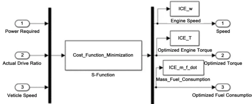
[image:5.595.108.525.328.426.2]The engine is modeled using an existing 3 L engine map to obtain a target gear ratio and a torque for given secondary pulley speed and throttle position. To derive the target
Figure 3. A block diagram showing the full system model, including driver, engine, CVT and vehicle road load models.
[image:5.595.80.553.457.690.2]gear ratio and torque output of the engine, a specific ratio set point strategy known as optimal operation line tracking is used.
The ratio set point determines the engine efficiency and also affects the drivability of the car. Thus careful consideration must be given to set the operating points depending on various road load demands and speeds. In this study, the ratios set points are chosen with the aim of minimizing fuel consumption. This is known as Optimal Operation Line Tracking (OOL Tracking). Although it optimizes fuel economy, it gives rather poor performance due to the limitation of the torque [4]. To set the ratio points first an S-Function is utilized, Figure 5, that optimizes the torques at each power line. This is done by using a cost function that minimizes fuel consumption [12], as following:
( )
0 min d
T f
J=
∫
m t t(1)
Subject to
• P=Preq
• P=Te∗we =mf∗Qlhv
• mf = f T w
(
e, e)(
Includes Efficiency)
• widle<we<wredline
• Te<Tmax
( )
weBy using the above-explained cost function; an optimum throttle versus speed map is derived by fitting a new line on the optimal operation line, Figure 6. This is done in order to achieve smooth drivability [13].
Optimized Torque Out Throttle Position
Maximum Torque
= (2)
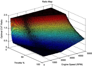
[image:6.595.106.549.503.686.2]Now using a constantly increasing velocity profile and the final drive ratio, the re-quired secondary pulley speed for each vehicle velocity is calculated. Using this sec-ondary pulley speed and optimal throttle for each speed and secsec-ondary pulley speed a map of the optimal CVT gear ratio is calculated, Figure 7. The system constraint is (Minimum Ratio ≤ CVT Ratio ≤ Maximum Ratio).
Figure 6. The optimal engine operating line (OOL) that minimizes the fuel consumption as a function of engine throttle and speed.
Figure 7. Optimal CVT ratio map as a function of throttle demand and engine speed.
4.3. CVT Model
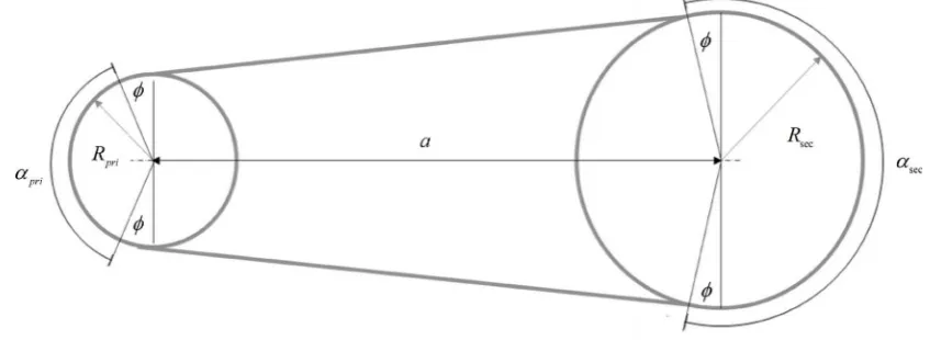
[image:7.595.196.549.378.629.2]va-riator will be displaced equally and oppositely by (Xp), leading to modified variator
radii and thus modified gear ratio. Assuming the total push-belt length is constant, the kinematics of the two variators are described by the nonlinear equations as following:
(
π 2)
(
π 2)
2 cos( )
0pri sec
R ∗ + φ +R ∗ − φ + ∗ ∗a φ − =L
(3)
( )
sin 0pri sec
R −R − ∗a φ = (4)
0 pri sec
R −R ∗GR= (5)
Here Rp, Rs and GR are the primary radius, secondary radius and the gear ratio
respectively.
φ
is the belt entrance angle, a is the center distance between the variators and L is the total belt length. Equation (3), can be derived by summing the belt lengths over the pulleys and in the free sections, which is equal to the total belt length (L). Ad-ditionally, Equations ((4) and (5)) describe the constant pulleys center-to-center dis-tance (a) as a function of the angle (φ
) and the pulleys gear ratio, respectively. Regard-ing the clampRegard-ing force actRegard-ing on the variator, this force between the belt and the varia-tor surface that is represented by:( )
cos 2 pri pri T F R β µ= (6)
The engine torque is given by T. Here it is assumed that the secondary clamping force is equal to the primary, without loss of generality, this assumption is adequate for the control problem objective, but it would be more accurate if the ratio between the primary and secondary force experimental data is available.
Thus, the forces acting on the variator including the hydraulic actuation force is giv-en as:
(
0)
primx=PA K x− −x −Cx−F
(7) [image:8.595.132.556.525.680.2]
Here m is the variator mass, P is the hydraulic pressure, K is the return spring stiff-ness, C is the damping coefficient and x is the variator displacement. Since the hydrau-lic circuit details are hard to obtain, and due to the fact, that the pressure rise and drop are linearly related to the solenoid input current, the pressure dynamics could be
Figure 9. Clamping forces (Fs and Fp) acting on the movable sheaves, input torque (Tp) and load torque (Ts) [14].
represented as a first order transfer function, with a time constant of 5 ms.
5. Hydraulic Control Strategy
The real CVT utilizes a current input to the hydraulic solenoid, and this is the main control input adopted in this model since the pressure is related to the variator dis-placement and accordingly to the variator radii and gear ratio. In the model it is as-sumed that both variators are displaced equally in opposite directions. From Figure 9, the primary variator displacement is related to the radius according to:
( )
, min2tan
pri pri
x
R R
β
= +
(8)
Since both variators are displaced equally, the secondary variator radius is:
( )
,max 2tansec sec
x
R R
β
= −
(9)
These two relations lead to a geometric gear ratio given by:
( )
sec( )
( )
priR x GR x
R x
=
(10)
sys-tem is stable and thus a PID controller should meet the control objectives such as fast response time (settling time) and minimized steady state error (to prevent gear ratio hunting or speed oscillations).
6. Results
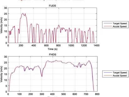
[image:10.595.199.497.296.355.2]A complete vehicle simulator including the pressure controller was constructed in Matlab-Simulink. The model was subjected to two driving cycles, namely Federal Ur-ban Driving Schedule (FUDS) and Federal Highway Driving Schedule (FHDS), to eva-luate the CVT and controller performances.
Figure 11 shows the vehicle actual velocity and the cycle target velocity. The results matches well with the target velocity meaning both the driver model and the available power were both capable of meeting the cycle-required load. Regarding the controller,
[image:10.595.141.554.372.681.2]Figure 12 depicts the target gear ratio needed to minimize the fuel consumption, as in-troduced in the model development section, and the actual gear ratio archived by the
Figure 10. Variator’s position-hydraulics PID controller.
Figure 12. Gear ratio tracking.
CVT pressure controller, both the desired and the actual are in good agreement. Notic-ing that the FUDS is mostly operatNotic-ing at higher gear ratios while the FHDS is at the lower gear ratios, this is due to nature of the driving cycle load and acceleration de-mands.
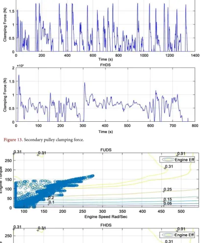
Due to the higher torque demands during FUDS cycle, the clamping force required is expected to be high due to proportional relation in Equation (6). This can be observed in Figure 13, which shows a higher required clamping force during FUDS than FHDS, therefore, it is most likely that the CVT parasitic load due to the hydraulic require-ments, during FUDS cycles or any similar driving behavior would be high.
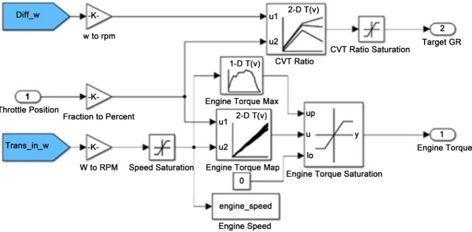
Figure 14 shows the operating points of the engine during the two driving cycles, it is clear that the CVT ratio controller is following the optimum operating line and it keeping the engine operating at the most efficient contours, this is regardless to the type of the driving cycle. However, during FUDS cycle, the engine operates at higher torque and speeds due to aggressive nature of the cycle velocity profile, while in the FHDS the figure shows fewer variations in the operating point due to the slowly varying speed profile of this cycle.
7. Conclusion
Figure 13. Secondary pulley clamping force.
PID that was tuned to provide a fast settling time and minimized steady-state error to present engine speed oscillations. The CVT pulleys were modeled as a mechanical hard stop, which represents the interaction between the CVT belt clamping force and the hydraulic pressure. The controller was implemented in a full vehicle model that in-cludes the engine, CVT, road load and a PID-type driver model. Two driving cycles were simulated and the results showed a good agreement in tracking the required ve-locity profiles as well as in tracking the optimum operating points.
References
[1] Srivastava, N. and Haque, I. (2009) A Review on Belt and Chain Continuously Variable Transmissions (CVT): Dynamics and Control. Mechanism and Machine Theory, 44, 19-41. http://dx.doi.org/10.1016/j.mechmachtheory.2008.06.007
[2] National Research Council (2015) Cost, Effectiveness, and Deployment of Fuel Economy Technologies for Light-Duty Vehicles. National Academies Press, Washington DC. [3] Bdran, S., Saifullah, S. and Shuyuan, M. (2012) An Overview on Control Concepts of
Push-Belt CVT. International Journal of Engineering and Technology,4, 392-395. http://dx.doi.org/10.7763/ijet.2012.v4.392
[4] Pesgens, M., Vroemen, B., Stouten, B., Veldpaus, F. and Steinbuch, M. (2006) Control of a Hydraulically Actuated Continuously Variable Transmission. Vehicle System Dynamics, 44, 387-406. http://dx.doi.org/10.1080/00423110500244088
[5] Kim, W., & Vachtsevanos, G. (2000). Fuzzy logic ratio control for a CVT hydraulic module. In Intelligent Control, 2000. Proceedings of the 2000 IEEE International Symposium on (pp. 151-156). IEEE.
[6] Bonsen, B., Klaassen, T.W.G.L., Pulles, R.J., Simons, S.W.H., Steinbuch, M. and Veenhui-zen, P.A. (2005) Performance Optimisation of the Push-Belt CVT by Variator Slip Control.
International Journal of Vehicle Design, 39, 232-256. http://dx.doi.org/10.1504/IJVD.2005.008473
[7] Wang, K., Zhang, X. and Zhong, Y. (2011) Research on the Ratio Control of Metal Belt CVT. 2011 International Conference on Electronic and Mechanical Engineering and In-formation Technology (EMEIT), IEEE, 7, 3485-3488.
[8] Ryu, W., Nam, J., Lee, Y. and Kim, H. (2005) Model Based Control for a Pressure Control Type CVT. International Journal of Vehicle Design (IJVD), 39, 175-188.
http://dx.doi.org/10.1504/ijvd.2005.008470
[9] Pfeiffer, F., Ed. (2008) Mechanical System Dynamics. Springer, Berlin.
[10] Ide, T., Udagawa, A. and Kataoka, R. (1995) Simulation Approach to the Effect of the Ratio Changing Speed of a Metal V-Belt CVT on the Vehicle Response. Vehicle System Dynam-ics, 24, 377-388.
[11] Bonsen, B., Klaassen, T.W.G.L., van de Meerakker, K.G.O., Steinbuch, M. and Veenhuizen, P.A. (2003) Analysis of Slip in a Continuously Variable Transmission. Dynamic Systems and Control, Volumes 1 and 2, 995-1000.
[12] Alzuwayer, B., Abdelhamid, M., Pisu, P., Giovenco, P. and Venhovens, P. (2014) Modeling and Simulation of a Series Hybrid CNG Vehicle. SAE International Journal of Alternative Powertrains, 3, 20-29. http://dx.doi.org/10.4271/2014-01-1802
[13] Hofman, T. and van Druten, R. (2004) Research Overview Design Specifications for Hybrid Vehicles. European ELE-DRIVE Transportation.
[14] Bonsen, B. (2006) Efficiency Optimization of the Push-Belt CVT by Variator Slip Control.
Nomenclature
req
P = Power requested by the driver. e
T = Engine torque. f
m = Fuel mass flow rate. ω = Engine speed.
lhv
Q = Fuel’s lower heating value.
, pri sec
R R = Radius of the primary and secondary pulleys.
φ
= Exit and entrance angle of the belt.a = Pulleys center to center distance.
L = Total belt length.
GR = Radii ratio.
F = Clamping force.
β
= Pulley half groove angle.µ = Coefficient of friction.
m = Variator mass. x = Variator displacement.
P = Hydraulic pressure. A = Variator piston area. K = Spring stiffness.
C = Damping coefficient.
Submit or recommend next manuscript to SCIRP and we will provide best service for you:
Accepting pre-submission inquiries through Email, Facebook, LinkedIn, Twitter, etc. A wide selection of journals (inclusive of 9 subjects, more than 200 journals)
Providing 24-hour high-quality service User-friendly online submission system Fair and swift peer-review system
Efficient typesetting and proofreading procedure
Display of the result of downloads and visits, as well as the number of cited articles Maximum dissemination of your research work
Submit your manuscript at: http://papersubmission.scirp.org/
![Figure 2. Schematic diagram for the pulley hydraulic control circuit [3].](https://thumb-us.123doks.com/thumbv2/123dok_us/7822518.731685/3.595.243.515.327.460/figure-schematic-diagram-pulley-hydraulic-control-circuit.webp)
![Figure 9. Clamping forces (load torque (Fs and Fp ) acting on the movable sheaves, input torque (T ) and pTs ) [14]](https://thumb-us.123doks.com/thumbv2/123dok_us/7822518.731685/9.595.252.496.67.331/figure-clamping-forces-torque-acting-movable-sheaves-torque.webp)