Munich Personal RePEc Archive
Causal misspecifications in econometric
models
Itkonen, Juha
ifo Institute for Economic Research, HECER
27 May 2011
Online at
https://mpra.ub.uni-muenchen.de/31397/
öMmföäflsäafaäsflassflassflas fffffffffffffffffffffffffffffffffff
Discussion Papers
Causal misspecifications in econometric models
Juha Itkonen
Ifo Institute for Economic Research and HECER
Discussion Paper No. 327 May 2011
ISSN 1795-0562
HECER
Discussion Paper No. 327
Causal misspecifications in econometric models*
Abstract
We bridge together the graph-theoretic and the econometric approach for defining causality in statistical models to consider model misspecification problems. By presenting a solution to disagreements between the existing frameworks, we build a causal framework that allows us to express causal implications of econometric model specifications. This allows us to reveal possible inconsistencies in models used for policy analysis. In particular, we show how a common practice of doing policy analysis with vector error-correction models fails. As an example, we apply these concepts to discover fundamental flaws in a resent strand of literature estimating the carbon Kuznetz curve, which postulates that carbon dioxide emissions initially increase with economic growth but that the relationship is eventually reversed. Due to a causal misspecification, the compatibility between climate and development policy goals is overstated.
JEL Classification: C50, Q54, Q43
Keywords: Causality, Policy evaluations, Energy consumption, Carbon dioxide emissions, Economic growth, Environmental Kuznets curve.
Juha Itkonen
Ifo Institute for Economic Research Poschingerstr. 5
81679 Munich Germany
e-mail: [email protected]
1. Introduction
To specify a model with causality is one of the most fundamental tasks of econometric policy analysis. Yet it seems that relatively little effort is put into developing analytical tools to help assess causality in econometric models and to gain insights on thea priori implications of different model specifications. The probabilistic language commonly used in econometrics does not provide a rigorous definition of causality. Therefore it is often exhaustingly difficult to debate about causes and effects in complex models with many equations, variables, and statistical assumptions.
Scientific discourse on causality requires a rigorous framework that al-lows to describe systematically, to break down, and to assess the meaning of various statements regarding causality between variables. Suchcausal frame-works allow to express well-defined causal statements that have well-defined truth values.
Different frameworks for handling causality have been developed (Hoover, 2008). The potential-outcome framework developed by Neyman (1935), Ru-bin (1974, 1978), and Holland (1986) is mostly used within statistics (Pearl, 2009; Heckman, 2005) and the program evaluation literature (Angrist and Krueger, 1999; Imbens and Wooldridge, 2009). It defines causality by an analogy with random experiments. Cowles Commission econometricians (Haavelmo, 1943, 1944; Marschak, 1950; Simon, 1953) defined causality with respect to structural equations models. The elaborate graph-theoretic frame-work by Judea Pearl (2009), which has received much attention recently, is partly based on the definition of causality by the Cowles group. The “econo-metric approach” for defining causality by Heckman (2005, 2008, 2010), and Heckman and Vytlacil (2007), which also builds on the Cowles Commission econometrics, has one crucial advantage over Pearl (2009) and the potential-outcome framework: it allows for simultaneous determination of variables (nonrecursive models and cyclic graphs) which is a property often needed in econometrics. The potential-outcome framework and Cowles Commission econometrics are considered to be special cases of Pearl’s framework (Pearl, 2009) and the econometric approach (Heckman and Vytlacil, 2007). Note that these interpretations of causality have little to do with predictive rela-tionship coined as Granger causality (e.g. Granger, 1969).
Pearl (2009). Causal ordering implied by a econometric model can be critical for the interpretation of the model. Visualizing causal relationships using graphs is not merely a way to illustrate a model, but also a tool for rigorous deduction.
Pearl’s framework has received some criticism by econometricians (Leroy, 2001; Neuberg, 2003; Hoover, 2003; Heckman, 2005; Heckman and Vytlacil, 2007; Heckman, 2008), with some resolved (Pearl, 2003; Pearl, 2009, p. 374– 380) and some left open. Its remaining weakness is the need to attach an unique dependent variable to each equation to define causality, which is sel-dom justified by economic theory.1
To get the best parts of both the econometric approach and Pearl’s frame-work, we build on a theory by Herbert Simon (1953) to establish a language to describe causal relationships and extract them from econometric models. We define a causal framework that fixes the aforementioned weaknesses in previous frameworks.
Our framework allows us to define and detect causal misspecification problems in econometric models. That is, it enables us to discover incon-sistencies within a wide range of models that are used for policy analysis. With these tools we can tackle problems in more complex models where they have been left unnoticed. We use the tools to show how policy analysis with vector error-correction models (VECM) (Engle and Granger, 1987) gives in-consistent and biased results under common practices (see e.g. Lütkepohl, 2005; Watson, 1994; Hamilton, 1994; Johansen, 1995). The problem is re-lated to the asymmetry of the cointegration rank tests.
To apply the tools into practice, we analyze a resent strand of literature estimating the carbon Kuznetz curve (CKC), which postulates an “inverted U”-shape relation between carbon dioxide emissions and aggregate output of economies. That is, emissions are assumed to initially grow with output, but the relation is reversed when the economy reaches a higher level of output. In this paper we discuss the problems related to the new strand of literature by focusing on the seminal work by Ang (2007). We argue, first, that the model includes an implicit constraint that is neglected in the estimation. Second, the causal effects are misinterpreted due to variable definitions. Third, the
1
model is biased to overstate the compatibility of development and environ-mental policy goals. In a more realistic model emissions rise quicker, peak later, and decrease slower as output increases.
It is our intention to strictly limit to the task of analyzing model specifi-cations and their consistency.2 We do not discuss identification, estimation, or testing, except to point out immediate implications regarding them, and to show the relevance of the theoretical considerations. Forgetting this dis-tinction is a source of much confusion (Heckman and Vytlacil, 2007; Pearl, 2009).
In the next section we present a framework for expressing causality. In the third section we introduce the new CKC literature, discuss Ang’s (2007) model, and derive an accounting identity that causes one of the problems. In the fourth section we describe the aforementioned three problems and apply the causal framework. In the fifth section we conclude.
2. Causal framework
Next we develop a framework for analyzing causality. We present the parts of the causal framework that are needed to show how common practice policy analysis with VECMs fails and to present the misspecification prob-lems in the new CKC literature. We build on the graph-theoretic, causal Bayesian network literature pioneered by Pearl (2009), but we take seriously the criticism made by econometricians (Leroy, 2001; Neuberg, 2003; Hoover, 2003; Heckman, 2005; Heckman and Vytlacil, 2007; Heckman, 2008) and adapt ideas suggested by Heckman and Vytlacil (2007). To define causality, we utilize and generalize the theory by Simon (1953) (which is also aug-mented by Simon and Rescher (1966); Simon and Iwasaki (1988); Druzdzel and Simon (1993)).
We define a causal framework that overcomes weaknesses in Pearl’s causal model and Heckman’s “econometric approach”, in order to enhance its suit-ability for econometric analysis. The main benefit is that we can analyze causality with graphs in models with simultaneously determined variables, such as the vector autocorrelation (VAR) model. Next we give a descriptive account of the distinctive features of our framework before giving a rigorous definition.
2
First, in order to analyze causality as defined in the Bayesian network literature, Pearl’s (2009) framework is limited to models with acyclic re-lationships, or recursive systems, which means there are no cycles of cau-sation. For such models, defining causal interpretations for parameters is less debated (Strotz and Wold, 1960, 1963; Basmann, 1963b,a). However, most econometric models are nonrecursive, i.e. some variables are deter-mined simultaneously by a set of equations, and there can be causal cycles. When variables are simultaneously determined, Pearl’s causal model can not be used. Pearl’s limitation to recursive systems has been the main point of criticism by econometricians (Leroy, 2001; Hoover, 2003; Neuberg, 2003; Heckman and Vytlacil, 2007).
We, however, are interested in thenecessary causal relationships implied by a econometric model, as we are looking for inconsistencies in model spec-ifications. Therefore we leave open the question of causality between simul-taneously determined variables and focus on what can be agreed upon. This allows us to extend the framework to nonrecursive models.
Second, nonrecursiveness of models implies that variables enter model equations symmetrically. This means we circumvent the so called matching problem, i.e. the need to identify one variable for each equation and consider that variable as the output (or the dependent variable) of the equation.3 Such matching has been a major obstacle for using Pearl’s framework in econometrics, since economic theory usually does not justify that there is a specific dependent variable for each equation of the model.4
Our way of avoiding the matching problem, however, makes it impossible to use Pearl’s definitions for interventions and counterfactuals. In Pearl’s framework interventions and counterfactuals are defined by “surgery” and “shutting down” equations (Pearl, 2009, p. 374). Anyhow, such model manipulations have received criticism from econometricians (Neuberg, 2003; Heckman and Vytlacil, 2007).
Third, in our framework interventions and counterfactuals are defined with variables that are determined outside the models (see Pearl, 1993, 2009, p. 70–72). The points of interventions are modelled explicitly and separately by defining a set of possible actions. We consider models as isolations and
3
Instead, we partition the sets of equations (derived substructures, defined later) and variables (which are solved in the derived substructures), and match between these subsets (see Dash and Druzdzel, 2008).
4
idealizations of the world (Mäki, 2011, 2008) and regard the economist as a deistic demiurge of the model world: first the economist defines the model that represents reality, next he chooses an action (a policy or a treatment) outside of the model, and then lets the model resolve itself generating an out-come. Consequently we manage without Pearl’s do-operator and “surgery”. We note that to choose nothing is also an action, and hence interventions can be defined equivalently using conditional probabilities or fixing (Pearl 2009, p. 70–72, Heckman and Vytlacil, 2007).
The action variables are strictly separated from other variables. Hence, the demiurge can never fix the same variables that describe the unit of ob-servation. For example, the price determined by the market is never quite the same variable as the price determined by the government. However, if justified, the model can be specified such that fixing an action to a particular value (government-set price) has the same result as if other variables (market price) realize with the same value. This strict separation of action variables and other variables is pivotal for defining interventions without model ma-nipulations like the “surgery”.
The econometric approach ends up doing surgery in a very implicit way, as argued by Pearl (2009, p. 374–380). One simply can not fix endogenous variables (to assess causal effects) when their value is uniquely determined by the set of model equations: If one changes the value of the outcome to something other than the solution, it results in a contradiction with the set of equations. By definition there is only one outcome that satisfies the set of equations. This somewhat trivial notion is often neglected in the literature. To assess the causal effect between endogenous variables, one needs to explicitly formulate and justify a new, consistent causal model, which isolates and idealizes reality in a way that the causing variable is an action variable.5 In our framework “surgery” can be expressed by specifying the points of intervention and action variables accordingly. That is, equations can be shut down with action variables if so specified. Moreover, we never end up contradicting with the initial model. The resulting framework is a slight generalization of Pearl (2009, p. 71).
Fourth, assuming symmetry between variables makes extracting a causal ordering slightly more complicated compared to acyclic models. We develop further the theory introduced by Simon (1953), known as thecausal ordering
5
algorithm, which defines a systematic way to express the asymmetric relation-ships between variables in a set of equations, relationrelation-ships that correspond to the conventional meaning of causality.6 That is, a set of equations related to a econometric model contains in its formulation a description of causal relationships, and Simon’s theory allows us to explicate this causal content. We generalize Simon’s (1953) theory into a non-linear and nonparametric form, we simplify it by adopting a new conceptualization, and proof that the causal ordering is unique.
Fifth, the main weakness of the econometric approach is its limitation to a simple dichotomic interpretation of causal ordering: variables are either effects or causes. Using causal graphs we can form a more complex picture where variables can be both causes of some variables and effects of others. Such a mesh of relationships can be easily depicted by a directed graph. This also obviates the need to differentiate between ex ante and ex post, or objective and subjective outcomes as done by Heckman and Vytlacil (2007); Heckman (2010).7
Our concept of “action variable” is similar to ”treatment“ in Heckman and Vytlacil (2007), except that a treatment can depend on other variables (for example in ”causal models for the choice of treatment“). In our frame-work such a model would be expressed by considering the treatment as an endogenous variable.
Sixth, because we only consider model specifications and set aside the other tasks of statistical inference, we can avoid a bountiful source of con-fusion by considering models simply as well-defined mathematical objects. Hence problems with policy invariance (as defined e.g. by Leamer, 1985; Heckman and Vytlacil, 2007),autonomy (as defined e.g. by Haavelmo, 1944; Aldrich, 1989; Pearl, 2009), and endogeneity (as defined e.g. by Wooldridge, 2002, p. 50–51) are not attributes of a single model, but are defined as a
relationships between two models. When considering bias, we need to
spec-6
Note that in this framework causality is defined in reference to a particular model specification, and does not necessitate causality in the real world nor include all forms of causality in theory: First, the framework itself is not subject to Hume’s critique, problems of observing causality, or any ontological problems (Simon, 1953). Second, determination of variables by definition is also defined as causal. Third, causal relationships between simultaneously determined variables are not determined. Here causality is simply a concept that proofs very useful in analyzing problems with model specifications.
7
ify the “true” and the “biased” model.8 A model is called “biased”, if there exists a better justified model, the “true” model, in which a given parameter of interest (e.g. the causal effect) has a different value. While postulating the “true” model, one also confirms that the offered specification is without contradictions.
Moreover individual models are always policy invariant and autonomous. That is, the parameters of a model do not vary because they are fixed by definition. If one wants to consider variation in these values, one needs to specify a model where they are defined as variables. Similarly models (as such) never suffer from endogeneity problems because all dependences between variables are to be specified by the model. This does not, however, imply that we only analyze “structural” models (in any sense of the word surveyed by Heckman and Vytlacil (2007)).
Furthermore, a causal parameter of interest might be infeasible in the “true” model, i.e. the parameter can not be defined in the “true” model without contradictions, even if it is well-defined in the “biased” model.9 In such cases the “biased” model does not just give distorted estimates, but the very existence of such an estimate is in logical conflict with the “true” model. This problem is far more severe than a simple case of poor approximation.
A weakness of our framework is that it is designed only for analyzing model specifications, so it makes no accommodations for identification, esti-mating, or testing. However it is clear that these tasks fundamentally depend on the soundness of the model specification.
We proceed as follows: first, we define a causal model which states the necessary specifications to consider causality in an econometric model, sec-ond, we show how to derive causal ordering between variables in a causal model, third, we show how to depict the causal ordering as a causal graph, fourth, we give an example, fifth we define causal effects and causal misspec-ification bias, and finally we consider the case of VECMs.
8
The idea is similar to the distinction between small and middle-size worlds by Simon and Iwasaki (1988). See also Mäki (2011).
9
2.1. Causal model
Let us consider astatistical model that consists of a set of random vari-ables W and a set of probability distributions P satisfying model equations
gi(w1, . . . , wn) = 0, i= 1, . . . , m, (1)
wheregi’s are real-valued functions; wj ∈W for allj = 1, . . . , n; andn ≥m.
Suppose we can partition the set W of a statistical model into disjoint subsets Y, X and U, where Y has m members. This could be called a econometric model (see e.g. Matzkin, 2007). Variables Y are observed and determined inside the model, and named endogenous; variables X are ob-served and determined outside the model, and are usually named exogenous; and variables U are unobserved and determined outside the model (as in Leamer, 1985). Here, we do not differentiate between unobserved and ex-ogenous variables, because they have identical roles when identification is not considered (Heckman and Vytlacil, 2007), hence we include unobserved variables in set X.10
The set of equations (1) can depict a structural model, a quasi-structural model, a VAR model, or something completely different. We consider these equations purely mathematical entities where the equality relation is symmet-ric. We do not implicitly differentiate between left and right hand variables. This results in a desired ambiguity between structural and non-structural models.
Note, that some variables entering functions gi can be trivial, i.e. not
all functions depend on all variables. This independence, as seen later, is actually essential for causality.
To consider the corresponding causal model, we first specify the points of intervention for the model. Interventions are done through a set of action variablesA, which specifies the ways the demiurge affects the model (actually or hypothetically). We define vector a∗
as a particular value of A which represents the action of making no intervention. We express the points of intervention with deep model functions fi, which correspond to model (1)
when a=a∗
, i.e.
fi(w, a∗) = gi(w)
10
is satisfied for all w = (w1, . . . , wn) and i.11 As a special case, we say
inter-ventions are additive if fi(w, a) = fi(y, x, a) = gi(y, x+a), where y ∈ Rm,
x, a ∈ Rn−m, and a∗
= 0. Under additive interventions, actions can be interpreted as changing the values of exogenous variables.
Next we define our fundamental concepts:
Definition 1. A set of equations S is a structure if it satisfies theregularity conditions:
1. S is uniquely solvable,
2. S contains an equal amount of equations and variables, and each sub-set of S contains at most as many equations as non-trivial, unsolved variables, and
3. S’s subsets are uniquely solvable if and only if they have an equal amount of equations and non-trivial, unsolved variables.
Let X and A denote the sets of possible values for the sets of variables
X and A, respectively.
Definition 2. Acausal model is a 5-tuple M = (Y, X, A, F, P), whereY,X, and A are sets of variables, F is a set of real-valued functions {f1, . . . , fm},
and P is a set of probability functions for variables X, if for all p ∈ P,
x0 ∈ X, and a0 ∈ A the set of equations
fi(y, x, a) = 0, i= 1, . . . , m (2a)
x=x0, (2b)
a=a0, (2c) is a structure when x0 is in the support ofp.
Compared to the plain statistical model, a causal model separates be-tween endogenous and exogenous variables, and specifies how interventions are done via action variables. Later we will see, that this provides the re-quired information to give meaning to causal statements.
The exogeneity equations (2b) and (2c) supplement the model equations
(2a) to state which variables are determined outside of the model. This is
11
Similar definitions are given by Heckman (2005) when naming the set of actions as possible treatments and functions fi as “deep structural” versions of gi, and by (Pearl,
required for an unequivocal causal ordering (Simon and Iwasaki, 1988) as shown later. Model equations (2a) and exogeneity equations (2b) and (2c) can be referred to as mechanisms. We emphasize that mechanisms do not necessarily relate to real world phenomena. Here a mechanism is just a name for equations of certain form.
Let vectorv(x, a)∈Rn denote the solution (or theoutcome) of structure (2) for given exogenous variables x ∈ X and action variables a ∈ A in causal modelM. We define interventions and counterfactuals in deterministic terms:
Definition 3. Given that x occurred, changing action from a toa′
has the effect of changing the outcome from v(x, a) to v(x, a′
).
Definition 4. Given that a was chosen and x occurred, the counterfactual statement “the outcome would have beenv′
if action a′
6
=awould have been taken“ is equivalent to saying v′
=v(x, a′
).
Counterfactual statements between arbitrary subsets of variables, i.e. “outcome of variablesV1 ⊂Y ∪X∪A would have beenv1, if V2 ⊂Y ∪X∪A had been v2 (given x)” are not well defined.12 To make such a statements, one has to add, how outcomev2 was achieved, i.e. define which action would
v2 as an outcome. In other words, one must specify the action a for which outcome v(x, a) is consistent with v2. Therefore the truth value of such sen-tences depends on how the counterfactual condition was reached. If no action results in outcome v2, such a sentence has no meaning in the given causal model.
We give an example to show how the concepts can be used. Consider a simple model equationg(y, x, u) =y−βx−u= 0, with endogenous variable
Y = {y}, exogenous variables X = {x, u}, and parameter β. Assuming additive interventions, we get a deep model functionf(y, x, u, a) = y−β(x+
a)−u. Now we get a causal model with a structure consisting of equation
y−β(x+a)−u= 0, x=x0, u=u0, and a=a0,
when (x0, u0) occurs and a0 is chosen. The resulting outcome of the model is a vector v(x0, u0, a0) = (β(x0 +a0) +u0, x0, u0, a0).
12
2.2. Causal ordering
The causal ordering of a causal model can be determined by studying the structure (2). The concept of structure is a convenient way to check whether sufficient and non-contradiction information is given to consider causation in an econometric model. The key innovation of Simon (1953) is that the order of solving the structure determines the causal ordering in the model. Roughly speaking, a variable is caused by all the variables that need to be solved to determine its value. Next we develop concepts to formalize this.
Definition 5. A subset of a structure is a substructure if it is solvable and does not contain any proper subsets that are solvable.
The following lemma states a property of substructures, that is important for showing that the causal ordering in a structure is unique.
Lemma 1. Substructures of a structure are disjoint.
The proof is presented in Appendix A.
LetS be a structure andsthe variables it contains. We can decomposeS
into two disjoint parts: First, we have S0 which is the union of all substruc-tures, e.g. S0 =S
1∪S2∪ · · · ∪Sk, whereSi is a substructure of structureS.
Second, we have the remainder R =S\S0.
Definition 6. Structure S is causally ordered if R is nonempty.
Definition 7. Let structureS =S0∪Rbe causally ordered and lets0 be the set of variables in S0. Now we can solve equations S0 to get unique values for variables ins0. By substituting the solved variables into setR we get the
derived structure of first order S1.
In less formal terms, the derived structure equals set R where solved variables s0 have been plugged in.
Under the first regularity condition, a derived structure must also be a structure. If it also is of causally ordered, its derived structure is called a derived structure of second order (of the structure S). By repeating, we can obtain the derived structure of kth order.
We proceed in this manner until the derived structure is not causally ordered, i.e. the remainder R is empty.
Definition 8. LetSkbe the derived structure ofkth order structureS. The
The substructures of the original structure are called the derived sub-structures of 0th order, and their union S0 is called the derived structure of 0th order.
Now structureShas been partitioned into disjoint subsets. We can denote
S =S0∪S1 = (S10∪S20∪ · · · ∪Sm00)∪S1
= (S10∪S20∪ · · · ∪Sm00)∪(S11∪ · · · ∪Sm11)∪S2
= (S10∪S20∪ · · · ∪Sm00)∪(S11∪ · · · ∪Sm11)∪ · · · ∪(S1n∪ · · · ∪Smnn),
where Sk is the derived structures of kth order, Sk
1, S2k, . . . , Smkk are the
de-rived substructures of kth order, mk is the number of derived substructures
of kth order, and n is the highest order of derived structures. More consisely we can write S =∪l
k=0∪m
k
i=1Sik∪Sl+1 =∪nk=0∪m
k
i=1Sik for any 0< l < n−1.
Lemma 2. The partition is unique.
The proof is presented in Appendix A.
Similarly the set of variablessin structureS has been partitioned accord-ing to the derived substructures in which they are solved. Due to regularity condition 3, each derived substructure with m equations must solvem vari-ables.
As variables are uniquely related to the derived substructures, we can use the ordering to define key concepts related to variables.
Definition 9. Let variables x and y appear non-trivially in a derived sub-structure of kth order of structure S. Let dx and dy be the lowest order of
derived substructure where variables x and y appear non-trivially, respec-tively. Then in structure S,
• if dx =dy, variables x and y are simultaneously determined, and
• if dx < dy =k, we say x is a direct cause of y.
We denote a direct causal relationship with the symbol “→”. Note that, the direct cause relationship is not yet transitive. Therefore we define the following:
Definition 10. Let s be the set of variables in a structure. Variable x ∈ s
is a cause of variable y ∈ s if there is a sequence of variables z1, . . . , zn ∈ s,
We define causal ordering of a structure as the set of all direct causal relationships between variables. With these definitions, as a corollary of Lemma 2, we get our main result:
Proposition 1. The causal ordering of a structure is unique.
This guarantees that the properties of the causal ordering relate to the structure unambiguously.
2.3. Causal graphs
Next we define a causal graph, which describes the causal ordering and which we can present visually.13 A causal graph consists of a set of nodes, which is the set of variables a in structure A, and a set of edges, which is the set of all variable pairs (x, y) for which x → y. Together these form a directed graph, where arrows represent direct causes. The graph is drawn such that the 0th order variables are in a column on the left, the 1th order variables are in the second column, and so on. To simplify graphs, we depict simultaneously determined variables by a left bracket, and unite all arrows leading to variables in these brackets (see Simon and Rescher, 1966).14
Now from Proposition 1 it immediately follows that a graph is a sufficient representation of the causal ordering of the structure:
Proposition 2. The causal graph of a structure is unique.
13
This is specified as a partial causal graphs in Dash and Druzdzel (2008).
14
2.4. Example
Lets look at an example to illustrate the framework. Let
f1(v1, v3, v5) = 0 (3a)
f2(v2, v3, v4) = 0 (3b)
f3(v3, v4, v5) = 0 (3c)
f4(v3, v4, v6) = 0 (3d)
v5 =a (3e)
v6 =b (3f) be a structure, where a and b are given. First, we see that equations (3e) and (3f) are substructures and form the derived substructures of 0th order. Therefore the structure is causally ordered. Variablesv5 and v6, which could be exogenous or action variables, can be solved and substituted in the other equations. Next, while v5 and v6 are now given, equations (3c) and (3d) can be solved simultaneously, but not separately. This means {(6b),(6c)} is the only derived substructure of 1th order. Therefore values for v3 and v4 are simultaneously determined. Finally, we are left with equations (3a) and (3b). They both form a derived substructures of 2th order. Solving them gives the value for v1 and v2.
With this information we can form a graph:
v5 ( v1 v3
v4
v6 v2.
(4)
In graph (4) we see, for example, that v6 is a cause of v1 and a direct cause of v4. The variables v5 and v6 are exogenous in the structure, and variables v1,v2, v3, and v4 are endogenous in the structure.
2.5. Causal effects and misspecification bias
variable in the “biased” model contradicts the “true” model (see an example below). Bias occurs when the magnitude of causal effect is different in the “true” and “biased” models.
To be more specific, we define the individual level deterministic causal effect of a change in an action for a causal model with continuous variables and differentiable model functions. The causal effect (CE) of action a ∈ A
on v ∈ Y ∪ X ∪A of a causal model is the total derivative dv
da. It can
be calculated from the structure of the causal model by using the implicit function theorem (or taking the total derivatives and applying the Cramer’s rule) (see Appendix B).
With additive interventions, an action a enters the functions similarly to it’s corresponding exogenous variable x ∈X. Therefore the derivative is same for both the action and exogenous variable. That is, for any variable
v ∈ Y applies dv
dx =
dv
da. This means we can analyze a model as if the
exogenous variables could be affected directly, which simplifies the causal model significantly. (An example will be given in Appendix F.)
For the rest of the paper we specify all models with additive interventions. Therefore we can analyze models as if the demiurge chooses the exogenous variables directly and omit the action variables from the structures and the causal graphs.
Let M1 = (Y1, X1, A1, F1, P1) be a “true” causal model with continuous variables and differentiable model functions with additive interventions.15 Now consider a similar “biased” causal model M2 = (Y2, X2, A2, F2, P2) such that there exists variablesx∈X1, X2 and y∈Y1, Y2. Suppose CE1 andCE2
are the causal effect of xon y in modelsM1 and M2, respectively. Then the
causal misspecification bias of the causal effect is CE2−CE1.
For example, such a bias emerges when the causal graph of the biased model does not include all causal paths from the effect x to the cause y. This occurs when the “biased” model incorrectly assumes a variable, z, as exogenous when it actually is endogenous such that x is a cause of z and z
is a cause of y. These missing paths, i.e. chains of arrows from x throughz
to y, are easy to detect from the causal graphs, as is with case of VECM.
15
2.6. Causal misspecification bias in VECM
Consider a vector autoregression model with three variables y1
t, yt2, and
y3t, one lag, and a error-correction representation ∆yti =b1iz1t−1+b2iz
2
t−1+εit, (5)
where εit are random disturbances;
∆yti ≡yit−yit−1 (6) are differences;
zt1 ≡a11yt1+a21yt2+a31yt3 (7)
zt2 ≡a12yt1+a22yt2+a32yt3 (8)
are error-correction terms for every time t = 0, . . . , T; and bji and ai j are
parameters for all i= 1,2,3 and j = 1,2. (See for example Hamilton, 1994, p. 580–582.) We call this model B.
Now consider a related model A, where equation (8) is substituted with
zt2 = 0. This corresponds to omitting the second cointegration equation from the model.
Finally, consider modelC, which is similar to model B in equations (5)– (8) but includes a third cointegration equation. Hence, equations (5) are supplemented with a third error error-correction term z3t.
We can summarize the three models by noting that they are all VECMs where the cointegration rank of model A, B, and C are 1, 2, and 3, respec-tively. That is, the models have a different number of cointegration equations included in them.
A common practice of doing policy analysis with VECMs is to consider a part of the model, called the long-run model (see e.g. Engle et al., 1989), which consists of equations (7)–(8) in the case of modelB, i.e. the cointegra-tion equacointegra-tions. When considering the long-run model, the error-correccointegra-tion terms,zti, are considered as exogenous error terms. Policy assessment is made by considering counterfactual statements with respect to these equations and evaluating causal effects between the variables.
The problem with the common practice is in the statistical test procedure (see e.g. Watson, 1994; Hamilton, 1994; Lütkepohl, 2005) based on Johansen (1988, 1995), to specify the cointegration rank. More specifically, the problem is with the tests for cointegration rank that are used to determine which cointegration equations (7)–(8) to include in the model. In the procedure, first, we justify the existence of one cointegration equation by testing the null hypothesis of no cointegration equations against the null hypothesis of one or more cointegration equations. If the null hypothesis is rejected, we infer that there must be at least one cointegration equation, in which case, we continue by testing the null hypothesis of one cointegration equation against the hypothesis of two or more cointegration equations. We continue in this way until the null hypothesis can not be rejected. Then policy evaluation is done with a model where all thus inferred cointegration equations are added. The test is more cautious not to make a false positive, i.e not to specify the model with cointegration equations that are not in the “true” model. Correspondingly, the test makes a false negative more often, i.e. fails to reject the null hypothesis when it is false. A false negative occurs especially often when the power of the cointegration rank test is poor, like when the sample size is small and deterministic trends are possible (Demetrescu et al., 2009). This unevenness accumulates so that the test procedure tends to result in a model with a too low cointegration rank.
However when considering causal effects, causal misspecification bias oc-curs symmetrically with a false positive and a false negative. That is, it is equally harmful to have too many or too few cointegration equations in the model. Hence the uneven test procedure is not well-founded.
We show this symmetry by considering models A, B, and C. First, let us consider the case of a false negative. Suppose that model B is the “true” model, i.e. the true cointegration rank is 2. Suppose that in the test proce-dure the first null hypothesis is rejected, but the second is not. Now we infer that equation (7) holds, but equation (8) might or might not hold, and drop it out of the model. This false negative results in modelA, which is “biased”. LetCEA and CEB be causal effects (for example between y1 and y2) in
models AandB, respectively. Now if we useCEA, instead of the true causal
effect CEB, we end up with causal misspecification biasCEA−CEB because
of the false negative.
cointegration rank is 2, add equation (8), and end up with model B, which is “biased”. In this case the causal misspecification bias is CEB−CEA, which
is equal and opposite to the previous case.
Furthermore, in addition to bias, there is the problem of infeasibility of causal effects. To see this, consider that the “true” model is modelC, which has three cointegration equations. Because there are only three endogenous variables, the three cointegration equations give a unique solution for the variables. Because the values are determined by the equations, we can not intervene with them without creating a contradiction. Hence, the causal effects between the variables can not be calculated, i.e. they are infeasible. If we make a false negative in this case and leave out cointegration equations, the analysis of causal effects is in logical contradiction with the “true” model. To conclude, because of the uneven treatment of false positive and nega-tive, the common practice fails to deliver unbiased estimates of causal effects. Moreover, a failure to detect a full cointegration rank leads to a logically in-consistent causal analysis.
In section 4 we show how bias emerges with the CKC literature, because of a missing equation.
3. Carbon Kutznets curve
3.1. The new approach
We apply the causal framework to analyze a recent strand of literature in environmental economics dealing with the long-standing debate on the environmental Kuznets curve (EKC), which has received novel attention as concerns for climate change and the need for global mitigation action have gained more awareness. The EKC depicts a relationship between emissions and output: at low levels of economic development growth increases emis-sions, but at higher levels of output the relationship is reversed. Graphically this implies an “inverted U” shape for the function of output to emissions (see Figure 1). When the focus is particularly on carbon dioxide emissions, the relationship is referred to as the carbon Kuznets curve (CKC).
9.0 9.2 9.4 9.6 9.8 10.0
1.8
1.9
2.0
2.1
2.2
2.3
Logarithm of GDP per capita
Logar
ithm of total carbon dio
[image:22.612.170.426.153.387.2]xide emissions
Figure 1: Relationship between the logarithm of per capita CO2emissions per capita and
the logarithm of per capita GDP in France, 1960-2006.
between development and mitigation goals, and a need for separate climate policies.
Over the last few decades the EKC-hypothesis has generated an enormous amount of literature. The recent strand of literature has attempted to merge the CKC literature (emissions-output-nexus) with a related topic concerning the relationship between energy consumption and output (energy-output-nexus)(See Figure 2).16
16
9.0 9.2 9.4 9.6 9.8 10.0
7.6
7.8
8.0
8.2
8.4
Logarithm of GDP per capita
Logar
[image:23.612.170.427.152.388.2]ithm of total energy consumption
Figure 2: Relationship between the logarithm of total energy consumption per capita and the logarithm of per capita GDP in France, 1960-2006.
We describe three problems concerning the foundations of this new strand of literature. First, the nonlinearity of the CKC model is not compatible with vector autoregression (VAR) models, because it creates a binding yet neglected constraint for the model, which compromises the integrity of the
estimators. The second and third problems relate to the inclusion of energy consumption as a explanatory variable.17 The second problem arises because emissions are not measured directly in the datasets that are used by the referred articles. Carbon dioxide emissions are defined by a linear function of different fuel commodities. As a result, controlling for the level of energy use means that only carbon intensity of energy is allowed to vary. Subsequently the interpretations of the parameters are very different. The third problem is caused by the dependence between energy use and output. When this dependence is recognized, we see that the model is biased.
In this paper we discuss the problems related to the new strand of litera-ture by focusing on the seminal work by Ang (2007). Some of the articles of the strand use slightly different methods and models so the problems mani-fest in different ways.18 But they all have the common feature of controlling for energy in a CKC model. As we restrict our analysis to the article by Ang (2007), we can only cast serious doubt on the validity of the other papers and motivate a need for a re-evaluation. It is then the task of another paper to assess their viability.
3.2. Ang’s model
Next we present the model introduced by Ang (2007). The CKC-hypoth-esis is examined using cointegration and vector error-correction modelling techniques (see e.g. Engle and Granger, 1987; Engle et al., 1989) applied to data on France between 1960 and 2000. The time series on emissions, energy use, and output are assumed to include stochastic trends, therefore many traditional time series methods are not applicable.
A long-run relationship between the time series can exist if stochastic trends are common to variables. A common stochastic trend implies that that there is a linear combination of the time series such that the combination is stationary. In which case, the time series are said to be cointegrated.
17
The articles in question only briefly comment the rationale for doing this. Some argue that it helps to tackle omitted variable bias, but, how it would solve the endogeneity problem, is left without any justification or discussion. Nevertheless, this is not a trivial matter, and is the source of the second and third problem.
18
Such a relationship is specified by Ang (2007) as a long-run (or steady-state) model
ct=β0+β1et+β2yt+β3y2t +ut, (9)
where ct is carbon dioxide emissions, et is total energy use, yt is real GDP
measured in local currency, all measured in per capita terms and converted into natural logarithms, and ut is a stationary error term.19
As in a typical CKC-model, the square of output is included to capture the nonlinearity in the CKC. The CKC-hypothesis implies that parameter
β2 is positive and β3 is negative to form an upside-down parabola. The novel feature is the included regressor et.
In addition to the long-run model, Ang (2007) studies the dynamic causal relationship between the time series by specifying a VAR model and the corresponding error-correction representation that incorporates equation (9). The VAR model describes how the variables vary, in the short-run, around the long-run model.
If Ang’s (2007) long-run model is to be used for policy analysis, the model must be interpreted causally. That is, to answer the central question of the CKC-literature (how does output affect emissions), we must be able to answer counterfactuals statements (if output was increased, how would emissions behave). In other words, we need a causal model.20
To consider the policy question of the CKC-hypothesis, the long-run model can be represented as a causal model with additive interventions. Its structure consists of equation (9) and of equations determining the value of the exogenous variables et, yt, and ut. Carbon emissions ct is chosen as
endogenous in order to answer policy relevant questions regarding the CKC-hypothesis.21 In this simple case, it seems that the carbon emissionsc
t is the
19
The long-run and short-run models are actually components of the same VECM. The error term of the long-run model corresponds to the error-correction term of the VECM. (Engle et al., 1989.)
20
Note that, even though Ang obviously refers with “causality” to Granger causality, the model must be appended with traditional causality if it is to have any policy relevance.
21
only endogenous variable. This can be depicted by a graph:
et
yt ct.
ut
(10)
In Section 4 we show that this causal ordering is not the full story.
To sum up, Ang’s model is policy relevant and attempts to address the CKC-hypothesis only if it is understood as a causal model where emissions are the effect of output. We claim that, if the model is interpreted in this manner, it can not answer the CKC-hypothesis. Note that we make no claims about causality in the real world. We are only interested about the consistency of causal statements with respect Ang’s model.
The following section will introduce the tools needed to present the prob-lems in Section 4.
3.3. The data and definitions
To consider the CKC literature, it is important to take into account how the carbon dioxide emissions data is produced in the datasets that are used in the literature.22 Essentially, there are no actual measurements of carbon dioxide emissions. They are simply calculated from energy statistics (see Appendix C).
We define an important concept: Carbon intensity Atis the average
emis-sions rate of energy consumption.23 Carbon intensity measures how much
22
Ang (2007), Apergis and Payne (2009, 2010), Soytas et al. (2007), Soytas and Sari (2009), and Jalil and Mahmud (2009) use data from the World Bank’s World Development Indicators (WDI) dataset, which in turn uses carbon dioxide emission data calculated by the U.S. Department of Energy’s Carbon Dioxide Information Analysis Center (CDIAC) (Boden et al., 2009). In the CDIAC dataset carbon dioxide emissions are calculated from consumed quantities of different fuel commodities and cement manufacturing. The CDIAC dataset uses energy statistics by the United Nations Statistics Division (UNSD) among others. UNSD data is used for the time period analyzed in this paper. The WDI dataset uses energy statistics compiled by the International Energy Agency (IEA). Richmond and Kaufmann (2006) use data compiled by the IEA on energy use, and calculates the carbon dioxide emissions by multiplying fuel use by the appropriate carbon content factor.
23
carbon dioxide emissions one unit of energy produces on average. Appendix C gives a formal definition.
Given the calculation form for carbon in the dataset and the concept of carbon intensity, we can derive identity
Ct≡EtAt+Xt, (11)
where Ct is carbon dioxide emissions, Et is total energy consumption, and
Xtis emissions from gas flaring and cement manufacturing, all measured per
capita. Appendix C shows how this identity is derived.
It is important to note, that this is simply an accounting identity derived from the definitions of the dataset, so it must be satisfied in the sample. That is, identity (11) holds by definition in the dataset.
To derive an algebraically more convenient form, we note that gas flaring and cement manufacturing amount only to a percent of total carbon emissions in the data, thus they can be omitted, i.e. set to zero. Therefore taking a natural logarithm of equation (11) gives
ct=et+at, (12)
where the variables are the corresponding logarithms of the capital letter variables.
Next we present the three problems in the new CKC literature and apply the causal framework.
4. The misspecifications in the new CKC literature
4.1. Transformations in a VAR model
The first problem arises because of the simple functional relationship between the observed variables yt and y2t. Inspired by Haavelmo (1943), we
notice that the system of equations implies a restriction between the joint distributions, which should have been taken into account in the estimation of the parameters. More specifically, the assumption of normally distributed i.i.d error terms (Johansen, 1988) is in contradiction with the VAR model equations.
To show this, lets look at the VAR model presented by Ang (2007):
xt=a0+
p
X
i=1
where xt = (ct, et, yt, y2t) is a vector of logarithms of observed variables, εt∈
R4 is a vector of error terms for time t = 0, . . . , T, a0 ∈ R4 is a vector of constants,Ai ∈R4×4 is a matrix of parameters for lagi, andpis the number
of lags.
To simplify the analysis, we restrict to a model only two variables,yt and
y2t, and assume that p= 1, a0 = 0, and Ai = [ajk]∈R2×2. Hence our model
consists of equations
yt=a11yt−1+a12yt2−1+ε1t and (14)
yt2 =a21yt−1+a22yt2−1+ε2t. (15)
Now plugging yt of equation (14) into equation (15) and rearranging gives
ε2t = (a11yt−1+a12yt2−1 +ε
1
t)2−a21yt−1−a22yt2−1. (16)
First,we notice that equation (16) constrains a polynomial relationship be-tween error termsε1t andε2t, hence they can not both be normally distributed, when the lagged variables are given at time t.
Second, we can show that the error terms are not independent over time. To see this, first note that equation (14) implies that ∂yt−1
∂ε1
t−1
= 1. Now using the chain rule and differentiating equation (16) gives
∂ε2t ∂ε1t−1
= ∂ε 2
t
∂yt−1
∂yt−1
∂ε1t−1
= 2(a11yt−1+a12yt2−1+ε
1
t)(a11+2a12yt−1)−a21−2a22yt−1,
which is generally non-zero. Hence the value of error term ε2t depends on
ε1t−1, and therefore they can not be chosen independently.
This means that the assumption of normally distributed i.i.d error terms, which is required by Johansen’s (1988) estimation method, can not be sat-isfied and the estimates are not reliable. We also see a much more general property: including a transformation of an endogenous variable into a VAR model as an endogenous variable creates an implicit constraint between error terms.
Alternatively, the problem can be seen easily by using the causal frame-work. First note that this VAR model specification does not constitute a structure if we assume that all error terms are exogenous. This is because, for each time periodt, we have two model equations but only one endogenous variable, as y2t is a simple transformation of yt. That is, given that the error
eachtbut only three variables,yt,ε1t, and ε2t. This means that the regularity
conditions are not satisfied and the equations do not form a structure, which implies that the model specification is inconsistent.
Instead, if we assume that one error term is endogenous, we get a con-sistent model. For this we can draw a causal graph that illustrates how the variables are determined:
ε21 ε22 · · ·
y0 y1 y2 · · ·
ε11 ε12
...
Here we clearly see, that error term ε1
1 is a cause of ε21 and ε22, which reveals the problematic dependency between the error terms. This is an example how the causal framework helps in detecting contradictions in the model setup.
Because there are other problems of misspecification in Ang’s model, on which we want to focus, we assume in the subsequent sections that the afore-mentioned problem is only minor and does not change the estimates signifi-cantly.
4.2. The interpretation of the parameters
Now we turn to the second problem. Wrong interpretation of the pa-rameters and resulting wrong conclusions arise from the definition of carbon emissions in the dataset (Section 3.3). It is worth emphasizing, that this problem is not about the fitness of the model, but is related to the specifica-tion of the model. We take Ang’s model as given in order to deduce what it actually implies.
In the context of CKC, the parameter of interest is the causal effect of output on carbon emissions. That is, we want to know how output effects emissions. In model equation (9), the proposed interpretation of the partial causal effect of yt on ct,
∂ct
∂yt
=β2+ 2β3yt, (17)
would be that it quantifies the causal relationship between emissions and output.24 This would be the Marshallian ceteris paribus change that assumes other variables constant (Heckman and Vytlacil, 2007).
This however, does not take into account the conceptual dependence be-tween energy and carbon emissions that is captured by identity (11). Recog-nizing this dependence reveals that the causal effect (17) has a much more narrow interpretation than implied.
Before applying the causal framework, we give, in more conventional means, three arguments for the existence of a problem, to show the necessity of a rigorous framework:
First, since the partial derivative (17) requires that total energy use et
is held constant, we notice from identity (11) that, in this case, the level of carbon dioxide emissions Ct can only change through changes in carbon
intensity At, or gas flaring and cement manufacturing emissions Xt. As the
significance of Xt is negligible and assumed zero, like in equation (12), a
change in output results in a change in carbon intensity at. The causal
ef-fect (17) can be interpreted only as the causal efef-fect of outputyton emissions
ctthrough carbon intensity at. This ignores the effect of yt onct through
en-ergy use et. As a result, the model is actually a regression analysis of carbon
intensity, instead of carbon emissions.
Second, the problem can be also seen by comparing the causal effect (17) and the derivative of identity (11). To simplify, assume gas flaring and ce-ment manufacturing emissions are constants. Now partially derivating iden-tity (11) with respect to yt gives
∂ct
∂yt
=et
∂at
∂yt
+ ∂et
∂yt
at. (18)
If emissions level et is held constant, as is required to calculate the causal
effect (17), the second term on the right hand side of (18) is omitted. This
24
means that the causal effect (17), which Ang (2007) investigates, is only the first term in (18).
Third, a more explicit regression equation can be formulated. When the negligible effects of gas flaring and cement manufacturing are assumed to be zero, equation (12) can be plugged into equation (9) to eliminate ct.
Rearranging gives equation
at =β0+ (β1−1)et+β2yt+β3y2t +ut. (19)
Here we see that model equation (9) is equivalently an regression on carbon intensity at, and the functional form between at and outputyt is exactly the
same as between carbon emissions ct and yt.
It easy to oppose this kind of reasoning with deceptively convincing coun-terarguments, by presenting different counterfactuals and relationships. To make a rigorous account of our argument and possible counterarguments, we use Simon’s theory.
First, we assume gas flaring and cement manufacturing emissions are zero for convenience. Second, we form a set of model equations
ct=β0+β1et+β2yt+β3y2t +ut, (20)
ct=et+at, (21)
where the first equation is (9), which is assumed to hold for arguments sake, and the second equation is (12), which result from identity (11) and the previous assumption. Third, we select the equations determining the value of the exogenous variables. This can be understood as fixing the inputs (see Heckman and Vytlacil, 2007). As exogenous we select variables et because
it is defined as a control variable, yt because it is represents our action, and
ut because it represents the other factors whose effect we want to omit as a
ceteris paribus assumption. We represent these by equations
et=e0t, yt=y0t, ut=u0t, (22)
wheree0t,yt0, andu0t are given values. We can think that the values are picked by some external mechanism, e.g. nature or the government.
the variables, which can be depicted as
et
yt ct at.
ut
(23)
Regarding the whole structure, carbon intensityatis the ultimate endogenous
variable. In other words, if a change in outputytcauses a change in emissions
ct, this means that carbon intensityat must have changed. This is not sound
with the theory of the carbon Kutznets curve because lower carbon intensity should be a cause of lower emissions, not the other way around.
Next show how the framework can be used to tackle some intuitive coun-terarguments. What if we claim that et is not exogenous and leave equation
et = e0t out? This would not be a structure any more and variables et, ct,
and at would not be determined. What if then choose ct to be exogenous
in-stead of et? Then we would get a different causal ordering and a new graph,
but this would not be relevant for inspecting the CKC hypothesis as we are interested in the effect of yt onct.25
What if we claim that there is an additional relationship between the variables? This means adding a new equation to the structure. This can give us a different causal ordering and a new graph. First, if the new equation contains a new variable, the effect is similar to adding equation (12) to model equation (9), as done above. Graph (10) corresponds to model equation (9) alone, but adding equation (12) gives us graph (23). Second, if the new equation does not contain a new variable, we have to make one variable endogenous. This is what we propose in the next section.
As we argued that Ang’s model is explaining carbon intensity instead of carbon emissions, one might wonder why the model fits so well. We ad-dress this question in Appendix E and argue the fit is misleading due to the polynomial shape of the model.
4.3. Bias
The third problem is a misspecification bias rising because energy use et
is dependent on output yt. To begin, let’s look at the data. First, note that
25
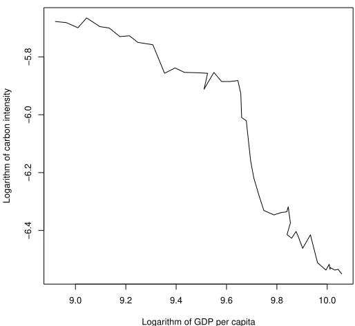
Figure 2 depicts levels of energy use over different output levels. It seems like there is a relationship between the variables: energy use is larger when output is larger. This suggest that producing more output requires more energy, as is apparent from theory. Second, note that, as identity (11) implies, variations in both carbon intensity and energy use are essential for the CKC. This can be seen from Figure 3. Here the development of carbon emissions in France (curve A) has been decomposed in to a growing energy consumption (B) and a declining carbon intensity(C).26 This shows that, without the growth of energy consumption, emissions in 2006 would be 60% less compared to 1960. On the other hand, without the shift to cleaner fuels, emissions would be 150% higher in 2006. This means that clearly both factors need to be accounted for.
1960 1970 1980 1990 2000
0.0
0.5
1.0
1.5
2.0
2.5
Year
Inde
x v
alue
B
A
C
Figure 3: Curve A is the index of carbon emissions, B is a index energy consumption, and C is the carbon intensity. By definitionA=BC.
26
To be more specific,A= ct
c1960,B = et
e1960, andC= ct
c1960/ et
The misspecification problem can be rigorously described by using the causal framework presented in chapter 2. The long-run model is the base of policy implications, and counterfactuals are stated with the long-run model equation (9). Therefore we can interpret the long-run model as a causal model and use the framework to show inconsistencies in the way causal state-ments are made.
We begin by first noting the three mechanisms dictated by the CKC-hypothesis and our knowledge of the definitions. These mechanisms describe how the variables relate to each other and allow us to construct a structure that can be compared to Ang’s structure.
First, we take into count the definition of carbon emissions in iden-tity (11). To clarify the results, we omit emissions from gas flaring and cement manufacturing, and use equation (12). This states that carbon emis-sions can be decomposed into carbon intensity at and energy use et.
Second, outputytis a cause of carbon intensity ataccording to the
CKC-hypothesis. This is also implied by Ang (2007) as shown in the previous section. Because we want to assess the bias in relation to Ang’s model, we assume that model equation (9) is satisfied.27 But because it actually describes a mechanism for carbon intensity at (as shown in the previous
section), we use the equivalent equation (19). In other words, we assume that equation (19) is satisfied to make a sensible comparison.28
Third, we note that also energy useet depends on output yt. This basic
notion, which is fairly evident (the details are the subject of the immense energy-output-nexus literature), is actually the motivation behind the strand of literature initiated by Ang (2007), and is essential to the CKC-hypothesis. Nonetheless it is unintentionally neglected due to the model formulation. To capture this relationship, we simply assume that there is a differentiable and monotonically increasing function e for which et = e(yt) +vt, where vt is a
error term.29
27
Note that we do not argue that this model is empirically valid in all respects. To the contrary, as we argue in Appendix E, carbon intensity is not a parabola. We construct our model to isolate one only one faulty aspect of Ang’s model, i.e. the bias, and focus on that.
28
Note that also equation (9) could be chosen but this would result in an unfounded causal ordering (presented in the previous section) without affecting the bias.
29
In addition, we fix yt because it represents our action variable, and we
fix ut and vt as ceteris paribus assumptions. This is denoted by equations
yt=yt0, ut=u0t, and vt =v0t.
These three mechanisms and three exogeneity equations form a set of equations, a structure with additive interventions,
ct =at+et (24a)
at =β0+ (β1−1)et+β2yt+β3yt2+ut (24b)
et =e(yt) +vt (24c)
yt =y0t (24d)
ut =u0t (24e)
vt =v0t. (24f)
The causal ordering of the structure (24) can be depicted by graph
vt et
yt ct.
ut at
The reasoning in the graph can also be expressed less formally. First, suppose yt, ut, and vt are determined by an external process, the economy
for example. Now also et is determined by yt and vt through the mechanism
(24c). When et, yt, and ut are known, using equation (24b), alsoat is
deter-mined. Now et and at are set, so carbon emissions ct is known by definition
with equation (24a).
Note that we could, for example, form the structure with model equations (9), (24a) and (24c)–(24f), but this would alter the causal ordering. As Si-mon (1953) show, this would be empirically indistinguishable from structure (24), even if it is theoretically invalid. In other words, the identification of the model is only partial. We choose the structure (24), from a set of em-pirically equivalent structures, because the resulting causal ordering is more reasonable. This, however, does not affect our main concern, the bias.