Munich Personal RePEc Archive
Futures basis, inventory and commodity
price volatility: An empirical analysis
Symeonidis, Lazaros and Prokopczuk, Marcel and Brooks,
Chris and Lazar, Emese
ICMA Centre, Henley Business School, University of Reading, UK
4 July 2012
Futures basis, inventory and
commodity price volatility: An
empirical analysis
∗
Lazaros Symeonidis, Marcel Prokopczuk,
Chris Brooks, and Emese Lazar
†July 4, 2012
Abstract
We employ a large dataset of physical inventory data on 21 different commodities for the period 1993-2011 to empirically analyze the behaviour of commodity prices and their volatility as predicted by
the theory of storage. We examine two main issues. First, we
explore the relationship between inventory and the shape of the forward
curve. Low (high) inventory is associated with forward curves in
backwardation (contango), as the theory of storage predicts. Second, we show that price volatility is a decreasing function of inventory for the majority of commodities in our sample. This effect is more pronounced
in backwardated markets. Our findings are robust with respect to
alternative inventory measures and over the recent commodity price boom period.
JEL classification: C22, C58, G00, G13
Keywords: Forward curves, inventory, commodity price volatility, theory of
storage, convenience yield.
∗We thank two anonymous referees, George Dotsis, Roland F¨uss, Apostolos Kourtis and
Chardin Wese Simen for helpful comments and suggestions. We also thank the participants at the Financial Management Association (FMA) European Conference 2012.
†ICMA Centre, Henley Business School, University of Reading, Whiteknights, Reading,
1.
Introduction
Over the past few years, the flow of funds to commodities has increased substantially, primarily through investments in exchange-traded funds (ETFs)
and commodity indices.1 This widespread interest in commodity investments
is partly associated with the view of commodities as a good diversification
tool, since their correlations with stocks and bonds have been low or negative (Gorton and Rouwenhorst, 2006; Buyuksahin et al., 2010). Recently,
Daskalaki and Skiadopoulos (2011) point out that these diversification benefits are preserved only during the recent commodity price boom (2003-2008), but in
their study vanish in an out-of-sample context. It is also a common belief that commodities provide a good hedge against inflation (Bodie, 1983; Edwards and Park, 1996). Moreover, recent evidence suggests that momentum and
term-structure based strategies in commodities can generate significant profits (Miffre and Rallis, 2007; Fuertes et al., 2010).2
The behaviour of commodity prices is strikingly different from that of stocks and bonds. For instance, such factors as seasonal supply and demand, weather
conditions, and storage and transportation costs, are specific to commodities and do not affect, or at least not directly, the prices of stocks and bonds. In
the light of these stylised facts, understanding the determinants of commodity prices and their volatilities is an issue of great importance.
The mainstream theory in commodity pricing, namely the theory of storage, explains the behaviour of commodity prices based on economic fundamentals.
Furthermore, it has major implications for the volatility of commodity prices. Since its inception, this theory has been the central topic of many theoretical
and empirical papers in the economics literature. Nevertheless, most studies employ proxies for inventory, such as the sign of the futures basis (e.g., Fama and French, 1988), thus providing only indirect evidence on the effect of
inventory on commodity prices and their volatilities.
In this paper, we employ real inventory data to test two of the main
predictions of the theory of storage. Specifically, we show how inventory affects
1
The Financial Times characteristically reports: “... inflows into the sector reached a new high of $7.9bn in October 2010, taking total investor commodity holdings to a record $340bn.”
2
the slope of the forward curve (the basis) as well as the price volatility for
a wide spectrum of 21 different commodities. Analyzing the relationship
between inventory and the term structure of futures prices is important for
various reasons. First, if inventory indeed has a significant effect on the shape
of the forward curve (“contango” vs “backwardation”), then it should also
affect the profitability of various term-structure based investment strategies.
Additionally, the strength of this relationship will provide further evidence on
whether the basis should be employed as a proxy for inventory in empirical
studies. Furthermore, the results from our research are of substantial academic
and practical interest since volatility underlies a variety of key financial
decisions such as asset allocation, hedging and derivatives pricing.
Our study contributes to the empirical literature on the theory of storage in
several ways. Gorton et al. (2007) employ physical inventory data to document
a negative non-linear relationship between inventory and the futures basis for
a large cross-section of commodities. They do not examine the link between
inventory and volatility in detail as we do. Also, Geman and Ohana (2009)
examine the relationship between inventory and the adjusted futures spread
in the oil and natural gas markets, using end-of-month inventory data. The
present paper adds to the evidence of the aforementioned studies by thoroughly
analyzing the link between real inventories and the slope of the forward curve
at several different maturities whereas previous research has only examined
the short end of the curve. Furthermore, the sample used for our analysis
includes the recent commodity price boom, which offers a great opportunity
to test our hypothesis over varying market conditions (for an analysis of the
recent commodity price boom, see Baffes and Haniotis, 2010).
Second, and more importantly, using our extensive inventory dataset, we
document a negative relationship between inventory and commodity returns
volatility. We characterise the time series variability of futures returns and
spreads with respect to inventory levels for each individual commodity. From
this perspective, our analysis is related to Geman and Nguyen (2005), who
analyze the relationship between scarcity (inverse of inventory) and returns
commodities as an asset class (Erb and Harvey, 2006; Brooks and Prokopczuk,
2011; Daskalaki et al., 2012), it is quite intuitive to examine the
inventory-volatility relationship for a broader set of commodities. For example, Fama
and French (1987) find that the implications of the theory of storage are not
empirically supported for certain commodities.
Our analysis provides a number of interesting results. First, we find a
strong positive relationship between logarithmic inventory and the slope of
the forward curve, the latter approximated by the interest-adjusted basis at
different maturities. In particular, lower (higher) inventory for a commodity is
associated with lower (higher) basis and forward curves in “backwardation”3
(“contango”) as the theory of storage predicts. Since the interest-adjusted
basis represents storage costs and convenience yields, our findings provide
insights regarding the relationship between convenience yield and inventory.
Our research also implicitly builds on the competing “hedging pressure”
literature, which is based on the existence of a risk premium earned by investors
in futures for bearing the risk of spot price changes. Recent empirical evidence
has shown that there exists a link between futures basis and risk premiums
(Gorton and Rouwenhorst, 2006).
Second, we find that price volatility is a decreasing function of inventory
for the majority of commodities in our sample. To do this, we estimate
for each commodity univariate regressions of monthly price volatility against
end-of-month inventory. Monthly price volatility is measured by the standard
deviation of daily nearby futures returns/adjusted basis for each month. The
magnitude of the reported relationship appears to be higher for commodities
that are more sensitive to fundamental supply and demand factors, which
determine storage. Moreover, heterogeneity is a possible explanation for
the difference in the sizes of the coefficients across individual commodities.
Some commodities are more difficult to store, and some of them are seasonal
3
or perishable, while others are not. Our evidence generally supports the
implications of theoretical studies (Williams and Wright, 1991; Deaton and
Laroque, 1992).
Lastly, we investigate the hypothesis that the effect of inventory varies
across different states of the market. To this end, we estimate OLS regressions
of commodity returns/futures basis volatility on the interest-adjusted basis,
decomposing the basis into positive and negative values that indicate the
state of inventories (positive basis – high inventory and vice versa). In line
with the implications of the theory, our estimation results suggest that the
relationship between inventory and volatility is stronger in backwardation
(low inventory). Furthermore, the results for energy commodities (crude oil
and natural gas) lend support for the existence of the asymmetric V-shaped
relationship between inventory and volatility reported by previous studies
(Kogan et al., 2009). For crude oil (natural gas), positive deviations from
the long-run inventory level (positive basis) have larger (smaller) impacts than
negative deviations of the same magnitude.
As mentioned in Gorton et al. (2007), there exist some problems when
dealing with inventory data. These are basically associated with the definition
of the appropriate measure of inventory (e.g. world vs domestic supplies) and
also with the timing of information releases regarding inventory levels. Another
potential pitfall concerns the difference in the quality of the corresponding data
from commodity to commodity, which hampers the ability to draw universal
conclusions. This is an inherent problem in any study that uses physical
inventories in the analysis. Therefore, any results using inventories should
be interpreted cautiously.
The remainder of the paper is organized as follows. Section 2 briefly
discusses the theory of storage and the relevant literature. Section 3
presents the datasets used for the empirical analysis. Section 4 examines the
relationship between inventory and the slope of the forward curve. Section 5
analyzes the relationship between scarcity and price volatility. Section 6 tests
the stability of the results obtained through various robustness tests. The final
2.
Theoretical background and relevant
liter-ature
The theory of storage, introduced in the seminal papers of Kaldor
(1939), Working (1948), Brennan (1958) and Telser (1958), links the
commodity spot price with the contemporaneous futures price through a
no-arbitrage relationship known as the “cost-of-carry model”. This theory
is based on the notion of “convenience yield”, which is associated with the
increased utility from holding inventories during periods of scarce supply. This
no-arbitrage relationship between spot and futures prices is given by:
Ft,T =St(1 +Rt,T) +wt,T −yt,T (1)
whereFt,T is the price at timet of a futures contract maturing at T,St is the
timet spot price of the commodity,Rt,T is the interest rate for the period from
t to T, wt,T is the marginal cost of storage per unit of inventory from t toT,
and yt,T is the marginal convenience yield per unit of storage.
Within the context of the theory of storage, convenience yield can be
regarded as an option to sell inventory in the market when prices are high,
or to keep it in storage when prices are low. Milonas and Thomadakis (1997)
show that convenience yields exhibit the characteristics of a call option with
a stochastic strike price, which can be priced within the framework of Black’s
model (Black, 1976). Evidence has also shown that convenience yield is a
convex function of inventories (Brennan, 1958; French, 1986).
A high convenience yield during periods of low inventory drives spot prices
to be higher than contemporaneous futures prices and the adjusted basis
becomes negative. Specifically, as inventories decrease, convenience yield
increases at a higher rate due to the convex relationship between the two
quantities. In contrast, at high levels of inventory, convenience yield is small
and futures prices tend to be higher than contemporaneous spot prices to
compensate inventory holders for the costs associated with storage. The theory
inventory. In particular, at low inventory states, the lower elasticity of supply
and the inability to adjust inventories in a timely manner without significant
costs (e.g., imports from other locations) make spot and futures prices more
volatile. As a result, basis also becomes more volatile. The opposite happens
at high inventory conditions.
Moreover, such factors as non-continuous production of some commodities
(e.g., agriculturals), storage costs, and weather conditions, exacerbate the
effect of demand shocks on current and future prices and thus have a significant
impact on price volatility.4 Fama and French (1987) use a dataset on 21
commodity futures and show that variation in the basis is driven by seasonals
in supply and demand, storage costs and interest rates. Also, Fama and French
(1988) employ the sign of the interest-adjusted basis as well as the phase of
the business cycle as proxies for inventory to analyze the relative variation of
spot and futures prices for metals. They find that when inventories are low,
the interest-adjusted basis is more volatile and also spot metal prices tend to
be more volatile than futures prices in line with the Samuelson hypothesis.
In a different version of the theory of storage, Williams and Wright
(1991) build a quarterly model with annual production and point out that
price volatility is highest shortly before the new harvest when inventories
are low. Deaton and Laroque (1992) suggest an equilibrium competitive
storage model, and show that conditional volatility is positively correlated
with the price level (the “inverse leverage effect”). Routledge et al. (2000)
develop an equilibrium model for commodity futures prices and show that
backwardation, driven by inventory and supply/demand shocks, is positively
related to volatility. A number of recent papers report an asymmetric V-shaped
relationship between inventory proxies and price volatility, meaning that both
high and low levels of inventory induce high price volatility (Lien and Yang,
2008; Kogan et al., 2009). Carbonez et al. (2010) provide contrasting evidence
on the existence of this V-shaped relationship in the case of agricultural
4
commodities.
The majority of the aforementioned studies employ indirect measures
for inventory, such as the (adjusted) futures basis to support their basic
arguments. Nevertheless, very few papers employ observed inventory data.
For instance, Geman and Nguyen (2005) construct a sample of US and global
inventories for soybeans at various frequencies and show that price volatility is
a monotonically increasing function of scarcity, the latter defined as the inverse
of inventory. Gorton et al. (2007) employ physical inventory data on a large
set of 31 commodities and conclude that the basis is a non-linear, increasing
function of inventory.
Apart from the theory of storage, the alternative view of commodity futures
prices, namely the hedging pressure hypothesis, is based on the idea of a risk
premium earned by long investors in commodity futures. According to the
very first version of the theory (Keynes, 1930; Hicks, 1939), speculators earn
a positive risk premium for bearing the risk short hedgers (producers) are
seeking to avoid. Later extensions show that producers can take both long
and short positions (Cootner, 1960), inducing risk premiums that vary with the
net positions of hedgers. This literature suggests that hedging pressure arises
from the existence of frictions (transaction costs, limited participation, etc),
which cause segmentation of commodity markets from other asset markets.
Another strand of the same literature relates risk premiums to systematic risk
factors based on the traditional CAPM (Dusak, 1973) or CCAPM framework
(Jagannathan, 1985; De Roon and Szymanowska, 2010). Finally, later studies
allow risk premiums to depend on both systematic risk and the positions of
hedgers (Hirshleifer, 1989; Bessembinder, 1992; De Roon et al., 2000) and
provide evidence that risk premiums vary with net hedging demand. In general,
the existence of risk premiums in futures prices and their determinants has been
a debatable issue among academics and practitioners.
It is therefore evident that gaining insights on the determinants of
commodity prices and their volatility is an issue of paramount importance,
not only for academics and practitioners, but also for policy makers (Bhar
dynamic relationship between commodity spot prices and their volatilities.
Furthermore, the issue of whether and under which conditions investors should
include commodities in their portfolios still remains an open question. Bodie
and Rosansky (1980) argue that including commodities in a portfolio of stocks
improves the risk-return profile of a typical investor. In contrast, Daskalaki and
Skiadopoulos (2011) cast doubt on the diversification benefits from investing in
commodities and find that these benefits exist only during periods of infrequent
bursts in commodity prices.
Moreover, some recent empirical work has focused on the so-called
“financialization” of commodities. This term indicates the increase in
co-movements of commodities with other assets (e.g. Silvennoinen and Thorp,
2010) or between seemingly unrelated commodities (Tang and Xiong, 2010).
This effect is widely considered a consequence of the increased participation
of new commodity investors and primarily hedge funds. Buyuksahin and Robe
(2010) argue that the positions of traders, especially hedge funds, led to the
recent increase in commodity volatility and comovement of commodities and
equities beyond what can be explained by macroeconomic fundamentals. This
is an issue of great importance for global policy makers since the increase in
volatility and comovement can exercise upward pressure on food and energy
prices, raising inflation concerns.
3.
Data and preliminary analysis
3.1.
Price data
The primary datasets employed in this study consist of daily futures prices
with several maturities for 21 commodities traded on the major US commodity
exchanges (NYMEX, CBOE, CBOT and ICE) and the London Metal
Exchange (LME). The full dataset covers the period from 31 December 1992
to 31 December 2011. The dataset for our analysis begins at the end of 1992
because this corresponds to a common starting point of most inventory series
in our sample. The particular commodities are selected to cover, as far as
metals. All price series except for metals are obtained from the Commodity
Research Bureau (CRB), which assembles data from all major commodity
exchanges worldwide. Metal price data are collected from Bloomberg. All
prices are expressed in US dollars. Since our study involves calculation of the
futures basis, we need the prices of futures contracts with different maturities.
The number of available maturities varies across different commodities from
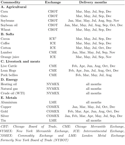
four to twelve per year. Table 1 contains a description of the commodity price
dataset.
For the purpose of our analysis, prices of the first nearby futures contract
are treated as spot prices, similar to Geman and Nguyen (2005). Since futures
contracts have fixed maturity months, we need to construct a continuous series
of futures prices for each commodity. To avoid expiration effects (Fama and
French, 1987) and low liquidity effects due to thin trading, we roll over from the
nearest to maturity to the next nearest to maturity contract on the last trading
day of the month preceding delivery. Since we also need longer maturity
contracts to compute the futures basis, we apply the same procedure for the
futures prices of the second nearest to maturity contract and so forth. We then
calculate the return of commodityi on dayt as the daily change in logarithmic
prices:
ri,t =log(
Fi,t,T
Fi,t−1,T
) (2)
whereFi,t,T is the closing price on dayt of the futures contract on commodityi
maturing atT. In calculating the returns we exclude the prices of the first day
of each delivery month in order to ensure that the computed returns always
correspond to contracts with the same expiry date (see, Fuertes et al., 2010).
Table 2 provides summary statistics for the daily nearby futures returns
series. Means and standard deviations of each series are expressed annualized
and as percentages. As seen from the table, the mean annualized returns of
metals and crude oil are the highest overall. Also, most of the agricultural and
animal commodities had negative average daily returns during the time period
considered. However, the result of a t-test fails to reject the null hypothesis of a
for all commodities. This is consistent with evidence in Erb and Harvey (2006).
Among the main drivers of this high price volatility are: the non-continuous
production of some commodities (e.g., agricultural), storage costs (Fama
and French, 1987), weather conditions (Geman, 2005), especially for the
agricultural and energy commodities, as well as the uncertainty regarding the
future macroeconomic conditions (e.g., changes in inflation, exchange rates
fluctuations, etc). Overall, gold exhibits the lowest amount of annual variation.
The annualized daily volatility of 47.39% for natural gas is the highest among
all commodities in our sample, followed by 39.24% for coffee. Crude oil and
heating oil nearby returns also exhibit significant amounts of daily variation
(33.7% and 32.1% respectively).
The sign of skewness is mixed, yet it is close to zero for most commodities.
However, the kurtosis coefficients are all significantly higher than three (except
for lumber), a standard evidence of non-normality. These non-Gaussian
features of commodity returns are also confirmed by the Jarque–Bera test
statistic, which clearly rejects the null hypothesis of normality in all cases.
3.2.
Inventory data
Apart from the commodity price data, we also compile a large set of inventory
data, using various sources. Most datasets correspond to end of month stocks
covering the period from December 1992 to December 2011. In those cases
when the inventory level is reported on the first day of a calendar month, we
shift to the end of the previous month. For some commodities, inventory data
are not available from 1993 (soybean oil, cotton, coffee, aluminium and tin)
and thus we utilize the subsequent date when those became available as the
starting point of our series. Also, due to the non availability of reliable data
for oats after 2003, we stop our sample at the end of 2003 for this specific
commodity. The data for agricultural and animal products are obtained from
the US Department of Agriculture (USDA). For soybeans, corn, oats and
wheat, the original datasets are available at a weekly frequency and thus we
consider the inventory level of the last week of month as a proxy for end of
US Energy Information Administration (EIA). Finally, data for metal stocks
stored in the Commodity Exchange (COMEX) for gold, silver and copper, and
the London Metal Exchange (LME) for aluminium and tin, are collected from
Datastream.
As discussed in Gorton et al. (2007), there are some problems when dealing
with inventory data. The first of those concerns the appropriate definition
of inventory. For example, in a global market such as that for crude oil,
international inventories may provide a better proxy for available supplies
compared to inventories stored at the various delivery locations across the
US. However, in a recent study, Geman and Ohana (2009) provide empirical
evidence that using either domestic US or global petroleum inventories leads
to very similar conclusions. Geman and Nguyen (2005) also find that
the relationship between inventory and spot price volatility for soybeans is
significant regardless of whether US or world soybeans inventory is employed.
Moreover, one can argue that a proper definition of inventory should take
into account all quantities that can be effectively used in case of a shortage,
including government or off-exchange stocks. Another problem is that in some
cases inventory data are released with a lag and are sometimes revised later.
This may create a problem when synchronizing these data with asset prices.
To alleviate the first concern, in the case of oil we employ some additional
measures for inventory, such as the volumes of all petroleum products in the US
and OECD countries. We also consider global inventories for corn, soybeans
and wheat in addition to domestic US inventories. Unfortunately, we lack
availability of global inventory data for the remaining commodities in our
study.
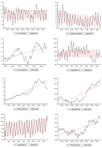
Figure 1 plots the inventory series for a subset of commodities along with
the fit of a seasonal function where applicable. An inspection of the graphs and
of inventory datasets reveals that the inventories of agricultural and animal
commodities, as well as those of natural gas and heating oil, exhibit strong
periodicity. To formally test for seasonality in inventories, we regress the
inventory of each commodity on monthly dummy variables. We then use the
each regression. As expected, corn, soybeans, and wheat exhibit very strong
seasonal variation, which is mainly driven by their non-continuous production
(crop cycles) and also by exogenous factors, such as weather conditions. Most
of the agricultural commodities in the domestic US market are harvested once
a year, and thus their inventory level reaches its peak immediately after the
harvest and is lowest shortly before the beginning of the new harvest.
Natural gas and heating oil stocks are also highly seasonal. This seasonal
variation is basically determined by higher demand during heating seasons
(cold winter months) combined with capacity constraints of the available
systems. Animal commodities (cattle, hogs and pork bellies) also produce
strong evidence of seasonality in their inventories. Seasonals in production,
perishability as well as seasonal variations in slaughter levels are among the
main drivers of this seasonal pattern. On the other hand, soybean oil inventory
does not exhibit seasonals, most likely because of its conversion process from
soybeans.
Also coffee, cotton, cocoa and lumber do not provide any evidence of
seasonal inventories. For the first two, this is most likely because of their
production process. For lumber, a possible explanation is that its demand is
determined by longer term factors, such as manufacturing activity and also its
production is more easily adjusted to demand (see, Fama and French, 1987).
Finally, metal stocks are not subject to short-term seasonal variations, since
there is noa priori reason for seasonality in supply or demand. Finally, crude
oil is continuously produced and consumed, and thus its stocks are not subject
to seasonal variations.
Our subsequent analysis is based on the logarithm of inventory to capture
the non-linear relationship between inventory and convenience yield/basis
documented by well-established studies (e.g., Telser, 1958; Deaton and
Laroque, 1992; Ng and Pirrong, 1994). We express our logarithmic inventory as
a deviation from the mean in order to remove the effect of measurement units
4.
Adjusted basis and inventory
Using our inventory dataset, we analyse the relationship between scarcity
and the slope of the forward curve individually for each commodity. The
forward curve slope is approximated by the interest-adjusted basis (henceforth,
adjusted basis) at three different maturities. Specifically, we construct the
series of adjusted basis for 2-, 6- and 10- month maturities. The theory
of storage implies that basis becomes more negative (positive) as inventory
decreases (increases).
In order to calculate the adjusted basis, we collect daily data on the
Treasury-bill (T-bill) yields of the corresponding maturities from Thomson
Reuters Datastream. We subsequently define the adjusted basis (bi,t) of
commodity i on dayt, as follows:
bi,t =
Fi,t,T2 −Fi,t,T1
Fi,t,T1
−Rf,tδ (3)
whereFi,t,T1 is the price on dayt of the first nearby futures contract maturing
inT1 days, which is used as the spot price in our study. Also, Fi,t,T2 is the time
t price of a futures contract with T2 days to maturity (T2 > T1) and Rf,t is
the annualised T-bill rate of the corresponding maturity on day t. δ = T2−T1 365
is the difference between the time to maturity of the two futures contracts
expressed in years. This difference is always as close as possible to the horizon
over which the basis is computed (i.e., 2, 6 or 10 months). Finally, bi,t is the
daily adjusted basis, which represents the slope of the forward curve on dayt. Since monthly data are employed for inventory in our framework, we further
adjusted basis for each month in the sample period.5
For three commodities (lumber, oats, and pork bellies), illiquidity of long
term future contracts did not allow calculation of the 10-month basis. In
general, an issue when calculating the basis concerns the fact that futures
contracts of different commodities do not expire every month. Thus, the
computed daily basis does not always correspond, for instance, to six months.
To address this, similar to Fuertes et al. (2010) and Daskalaki et al. (2012),
we take the price of the next futures contract whenever there is no traded
contract with six months to maturity. The same applies to the nearby futures
price treated as the spot price in our study. For instance, to calculate the
6-month basis of corn on 15 January, we need the price of the February
contract, maturing at the end of January, as the spot price, and the August
contract, maturing at the end of July, as the 6-month futures price. If there
is no February contract for this particular commodity, we consider the next to
maturity contract, i.e., the March contract, as the first nearby contract, and
therefore the September contract as the 6-month futures contract. Accordingly,
if there is no contract maturing in September for the specific commodity, we
consider the next to maturity contract (i.e., October), and so on.
4.1.
Empirical Evidence
Our first objective is to empirically test the relationship between inventory
and the slope of the forward curve (adjusted basis). To this end, we estimate
5
for each commodityi the following regression:
˜bi,τ =αi+βiI˜i,τ +ui,τ (4)
where ˜bi,τ is the deseasonalized forward curve slope of commodityi in monthτ,
computed as the monthly average of the daily adjusted basis of the respective
maturity (2-, 6, or 10-month) over each monthτ, and ˜Ii,τ is the deseasonalized
logarithmic inventory at the beginning of that month τ (or equivalently the end of month τ −1). The basis and inventories of some commodities exhibit seasonality. To deseasonalize these variables, we estimate regressions against
monthly dummies and use the residuals as the deseasonalized adjusted basis
and inventory in our regressions.6 A time trend is included in the seasonal
regressions of monthly logarithmic inventory when it is statistically at the 5%
level.
Adjustment for seasonality in the adjusted basis and inventory series of
each commodity is based on the significance of the F-test statistic, which
evaluates the null hypothesis that the coefficients of all monthly dummies are
equal. As a result, dummy regressions are not considered for metals, crude
oil, soybean oil, cotton, coffee and lumber, since there is no indication of
periodicity in either their basis or inventory. For these commodities, inventories
are expressed in deviations from their means to facilitate comparison across
different commodities and to remove the effects of measurement units.
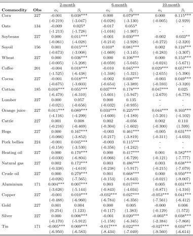
Table 3 presents the results from the univariate OLS regressions of equation
(4). Our results strongly support a positive and significant relationship
between inventory and the slope of the forward curve (adjusted basis) for all
maturities considered. More specifically, using a two-tailed test we conclude
that for the 21 commodities considered, 17 (18) coefficients are statistically
significant at the 5% (10%) level for the 2-month basis. The only exceptions
are lumber, cattle and gold. Moreover, the statistically significant coefficients
are positive in all cases. Adjusted basis for longer maturities (6, 10 months)
6
allow for very similar conclusions. This demonstrates the robustness of our
results with respect to the considered maturities.
Regarding the magnitude of the coefficients, we observe that all three
energy commodities and lean hogs exhibit the strongest link with inventory.
Overall, the largest in size coefficient is reported for crude oil, followed by
natural gas across all maturities considered. In particular, the coefficient
of the 6-month basis for crude oil is equal to 0.668. This means that a
deviation of 1% from the average inventory level for crude oil results in a
0.67% increase in the crude oil adjusted basis. The large coefficients for
energy commodities can be explained by high storage and transportation costs
as well as capacity constraints of available systems that deter storage and
make prices more sensitive to inventory withdrawals. An interpretation for
the strong significance in animal commodities could be the high storage costs
and perishability that lead to low inventory levels relative to demand. In
general, our results support the evidence of Gorton et al. (2007).
Apart from the energy and animal commodities, a strong association is
also observed for most of the agricultural and soft commodities. Significant
coefficients for these commodities are mainly related to the fact that most
of these commodities are harvested once or twice a year in the domestic
US market and the available inventory must satisfy demand over the whole
year. Given that total imports for these commodities represent a very
small proportion of annual production in the US, the prices of agricultural
commodities are highly sensitive to the levels of available stocks in the domestic
US market. Metals, and gold in particular, exhibit the lowest correlation
with inventory. The coefficient for gold is insignificant, while for the rest the
coefficients are usually very small in size (of order 10−3f orshort−termbasis).
Low storage costs relative to their value and sufficiently high inventory levels
relative to demand, especially for precious metals, are the main reasons for
these low correlations.
Also, in line with evidence in Geman and Ohana (2009), who used a slightly
shorter sample period (1993-2006), we find that the petroleum stock in OECD
(having a higherR2 coefficient). Moreover, the coefficient estimates for global inventories in respect of corn, soybeans and wheat are all highly significant at
the 1% level and their corresponding t-statistics are higher than those of US
inventories.
Overall, our results lend support to one of the main implications of the
theory of storage that inventory is positively associated with the slope of
the forward curve (the basis). Lower (higher) available inventory leads to
wider and more negative interest-adjusted basis and thus more backwardated
(contagoed) markets. Differences in magnitude across commodities are related
to their varying dependence on the fundamentals of storage. Our evidence is
robust for the forward slope at different maturities.
5.
Inventory and price volatility
Theoretical as well as empirical evidence on the theory of storage suggests
that price volatility is inversely related to inventory. For example, Deaton
and Laroque (1992) show in their theoretical model that next period spot
price volatility decreases with higher inventories. Also Ng and Pirrong (1996)
analyse the dynamic basis-volatility relationship in gasoline and heating oil
markets. Motivated by this strand of the literature, we use our physical
inventory data to directly test how inventory is related to subsequent
commodity price volatility. We distinguish between two alternative cases for
price volatility: i) adjusted basis volatility, and ii) the volatility of nearby
futures returns.
To obtain a measure for adjusted basis volatility, we first compute for each
commodity the annualised standard deviation from the daily adjusted basis
series for each monthτ. Then we estimate the following regression:
˜
σi,τ =αi+γiI˜i,τ +ϵi,τ (5)
where ˜σi,τ is the annualized standard deviation of the daily adjusted basis
series of commodity i in monthτ, and ˜Ii,τ is the inventory of commodityi at
deseasonalise both the inventory and the adjusted basis volatility as discussed
above.
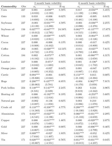
Estimation results are reported in Table 4. The coefficients of these
commodity-by-commodity regressions indicate a negative relationship between
inventory and adjusted basis volatility. Regarding the volatility of the 2-month
basis we see that for the 21 commodities considered, 14 (15) inventory
coefficients are statistically significant at the 5% (10%) level. From those 12
(13) are negative whereas two are positive. If we analyse the results across the
separate commodity groups, we see that the relationship is particularly strong
for most of the agricultural and energy commodities in terms of the sizes of
the regression coefficients. Specifically, all inventory coefficients are negative
and strongly significant at the 5% level in the agricultural commodity group,
except for oats.
Concerning the animal commodities, the coefficients for hogs and pork
bellies are statistically significant at the 1% level and quite high, although
of the opposite sign than anticipated (positive). This looks counter-intuitive
at first sight. However, a plausible explanation for this reversal in the
inventory-volatility relationship is that during periods of low demand when
inventories are usually high, the difficulty to increase storage due to capacity
constraints may lead to big price drops increasing price volatility. For the
animal commodities, this effect is further exacerbated by their perishable
nature. In an attempt to empirically test this line of reasoning we estimate the
same regression for hogs, decomposing deseasonalised logarithmic inventory
into negative versus positive values. The results indicate that the inventory
coefficient is positive for higher than average inventory, whereas it is negative
for lower than average inventory (a non-linear pattern).
From the three energy commodities, the coefficients of crude oil and heating
oil are both highly negative and significant at the 1% level. Surprisingly
given the sensitivity of its prices to storage levels, the coefficient of natural
gas is insignificant. However, the empirical evidence in Geman and Ohana
(2009) suggests that the negative inventory-volatility relationship for natural
scarcity), e.g. during winter. Indeed, if we estimate the same regression
separately for negative and positive values of deseasonalised inventory, we
observe a high negative correlation during periods of negative deseasonalised
inventory. Finally, the inventory coefficients of industrial metals are all
significant, whereas those of precious metals are always insignificant. The
absence of significance for precious metals does not come as a surprise since
variations in their prices are primarily determined by investment demand and
also inventories are sufficient in general to limit variations in convenience yields.
Also, the estimation results for the volatility of 6-month basis lead to very
similar conclusions.
Turning our focus to spot return volatility, we first compute for each
commodity the annualised standard deviations of daily nearby futures returns
over each month τ in the sample. The volatility series obtained are then employed as dependent variables in the following regression:
σi,τ =ωi+ζiI˜i,τ−1+ui,τ (6)
where σi,τ is the annualised standard deviation of the daily nearby futures
returns of commodity i over each month τ in the sample and ˜Ii,τ−1 is the
logarithm of inventory of commodity i at the end of month τ-1. Similar to the regressions of the adjusted basis volatility given by equation (5), we
deseasonalize inventory and nearby futures volatility by estimating regressions
against monthly seasonal dummies, as discussed above.
Estimation results are reported in Table 5. The coefficient on the inventory
variable is statistically significant for 11 (14) out of the 21 commodities
at the 5% (10%) level. Moreover, all significant coefficients are negative
except for those of hogs and pork bellies. Regarding the magnitude of the
coefficients, we observe that the relationship appears to be particularly strong
for energy, agricultural and animal commodities. The strong relationship
for energy commodities is mainly associated with high storage costs and
also with capacity constraints in production and transmission systems, which
commodities, on the other hand, the non-continuous nature of production,
significant storage costs and the inability to import supplies from other
locations during the cycle at a low cost, reduce the elasticity of supply and
thus increase the responsiveness of prices to supply and demand shocks. The
coefficient for soybeans is in consistent with Geman and Nguyen (2005).
Coefficients of hogs and pork bellies are significant, but positive. A possible
explanation is provided above. Finally, we observe relatively lower coefficients
for metals in comparison with the other commodities. The only notable
exception is copper, with a much higher coefficient relative to the other metals.
From metals group, only copper and tin provide support for a significant
relationship with inventory. This result for copper is most likely related to
the difficulty of storing this commodity.
Evidence from this last section suggests that commodity price volatility
is negatively associated with inventory fluctuations. However, this evidence
is not universal for all commodities because of their heterogeneity as an asset
class. For instance, some commodities such as the agriculturals are periodically
produced and therefore variation in inventory levels throughout the year affects
the sensitivity of their spot and futures prices to demand shocks. Gorton et al.
(2007) mention that high storage costs provide incentives to economise on
inventories and also limit the variation in available supplies. This can partly
explain the observed positive inventory-volatility relationship. The difficulty
in injecting into storage when demand is high and inventories sufficiently large
leads to a price drop and also to higher volatility. Energy commodities are
continuously produced and their prices are more demand driven. For example,
natural gas volatility is basically determined by demand shocks during the
heating season given the inability to increase production due to capacity
constraints of available systems. Gold, in contrast, is more of a financial than
a commodity contract as argued by many authors and therefore its prices
and volatility are expected to be more related to economic conditions (e.g.
inflation) than to inventory considerations. It is thus evident that the different
characteristics of each commodity affect the responsiveness of its prices to
and Harvey (2006), who observe significant differences in excess returns and
also in the sensitivity of these returns to inflation across various commodities.
5.1.
The effect of market states
Ng and Pirrong (1996) analyse the dynamics of gasoline and heating oil prices
and find that spot returns are more volatile in backwardation compared to
contangoed markets. Also, Fama and French (1988) show that the volatility of
metal prices is higher when interest-adjusted basis is negative. To test whether
this hypothesis is empirically supported by our data, we separate the adjusted
basis of each commodity into positive and negative values and then estimate for
each commodity two regressions using as dependent variable: i) the adjusted
basis volatility, and ii) the nearby futures volatility. The specification is:
σi,τ =ϕ0+ϕ1I{bi,τ−1>0}bi,τ−1+ϕ2(1−I{bi,τ−1>0})bi,τ−1+ei,τ (7)
where: σi,τ is the nearby futures/the adjusted basis volatility, respectively, of
commodity i in month τ and I{bi,τ−1>0} the indicator function that takes the
value of 1 if the 2-month adjusted adjusted basis of the previous month (τ−1) is positive and 0 otherwise, and bi,τ−1 is the adjusted basis of commodityi at
the end of monthτ−1. Therefore, if negative basis has indeed a larger impact on volatility, then we expect the coefficient of the negative basis (ϕ2) to be
significant and higher in absolute value than the corresponding coefficients of
the positive basis.
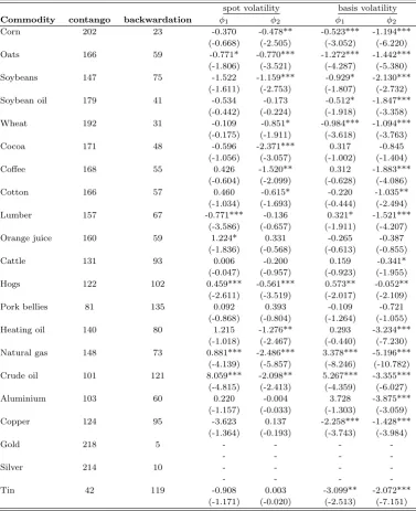
The results are presented in Table 6. Columns 2 and 3 report the number
of months in backwardation and contango for each commodity. We see that
the majority of commodities were mostly in contango. The only exceptions are
crude oil, pork bellies and tin. This observation for crude oil is in accordance
with Erb and Harvey (2006). Columns 4 and 5 contain coefficient estimates
when nearby futures volatility is employed as the dependent variable in the
regressions, whereas columns 6 and 7 report estimates for basis volatility as the
dependent variable. We exclude gold and silver from the analysis since their
between the impact of negative from positive basis. Again, the observation of
contango market for precious metals is consistent with Erb and Harvey (2006).
The results for nearby futures volatility support, in general, a stronger
link between inventory and volatility during backwardated markets. This
effect seems to be more pronounced for agricultural and soft commodities, for
which most positive basis coefficients are insignificant, whereas the negative
basis coefficients are negative and significant. Exceptions are soybean oil
and orange juice, where the coefficients are not significant in any case.
Significance is also absent for industrial metals. In addition, results for the
three energy commodities are of particular interest. Specifically, for crude
oil and natural gas, the results provide support for an asymmetric V-shaped
relationship between inventory and volatility, with both positive and negative
basis inducing higher volatility, consistent with previous studies (e.g. Kogan
et al., 2009). For crude oil (natural gas), positive basis has a larger (smaller)
impact than negative basis of the same size. Finally, among the three
animal commodities, only hogs provides significant estimates which supports
a V-shaped relationship. For heating oil, only the coefficient on negative basis
is significant at the 1% level.
For basis volatility, where the basis is defined as the difference between
the first and the second nearby futures contracts in excess of the interest rate,
we obtain slightly different results. Coefficients for many of the agricultural
commodities are now significant and negative in contango states, supporting
a universally negative correlation between inventory and volatility. However,
negative basis coefficients (backwardation) are always higher in absolute value
than those for positive basis (contango) of the same magnitude. From
the soft commodities, coffee and cotton provide significant coefficients only
in backwardation states, whereas cocoa and orange juice do not provide
significant coefficients in any state. The coefficients for energy commodities
lead to very similar conclusions to the case of nearby futures volatility. Finally,
copper and tin support a globally negative relationship with inventory in
contrast to the case of nearby futures volatility, where only the coefficients
6.
Robustness analysis
We perform a series of tests to check the robustness of the results obtained in
the previous sections. First, to check the stability of our results, we repeat
our estimations using sub-samples. Initially, we divide the entire sample
of each commodity into two equal sub-samples and re-perform the relevant
estimations. Apart from a few cases, our results are robust across the two
sub-periods considered.
The rapid growth in commodity prices between 2003 and 2008 provides a
motivation to analyze our main empirical relationships over this period and
to test whether any significant structural change occurred. We thus separate
our full sample in two sub-periods: 1993-2002 and 2003-2008, and re-perform
our estimations. The results over the commodity price boom period are very
similar to those obtained for the 1992-2002 period, as well as for the full sample
period and in some cases are even stronger. This provides some evidence that
variations in fundamental supply and demand factors continued to play an
important role during the period of sharp rises in commodity prices in addition
to the effect of increased participation from commodity index investors (Irwin
and Sanders, 2011).
Second, to provide additional evidence regardless of distributional
assump-tions, we perform all significance tests in our analysis additionally using a
non parametric test, Spearman’s rank order correlation. This technique is
distribution independent. Our results remain qualitatively similar.
Lastly, we test the relationship between inventory and the slope of the
forward curve using the 12-month adjusted basis as a proxy for the slope of the
forward curve. We compute the 12-month basis from equation (3) considering
the first nearby as well as the year ahead futures contract. The 12-month basis
has the advantage that it implicitly takes seasonality into consideration, since
taking the difference between the nearby and the year ahead futures prices
is similar to applying seasonal differences. Overall, our estimation results
7.
Conclusions
This paper analyses the fundamental role of inventory in explaining commodity
futures prices and their volatilities within the economic framework of the
theory of storage. Using an extensive dataset of monthly inventories for 21
different commodities for the period from 1993 to 2011, we empirically test two
of the main predictions of the theory of storage. First, we document a negative
relationship between inventory and the slope of the forward curve. The latter
is approximated by the interest adjusted basis at different maturities, namely
2, 6, 10 and 12 months, respectively. In particular, lower inventories are
associated with wider and more negative futures basis and therefore more
backwardated forward curves. This result also implies that the convenience
yield is an increasing function of inventory. Moreover, our evidence suggests
that (adjusted) basis can serve as a sufficiently good proxy for inventory in
empirical studies. These results also provide further support to those in Gorton
et al. (2007).
Second, in line with the implications of the theory of storage, we find
that inventory is negatively related to commodity price volatility. More
specifically, price volatility is a decreasing function of inventory. The
documented relationship appears to be stronger for energy, animal and
agricultural commodities and weaker for metals, and especially for precious
metals. Furthermore, conditioning our analysis on market states (contango
vs backwardation) we observe that a negative basis (low inventory) has a
more pronounced impact on volatility than a positive basis (high inventory).
Also, for energy commodities we document a V-shaped relationship between
volatility and the slope of the forward curve, consistent with previous empirical
studies (see, Kogan et al., 2009). These findings are preserved during the recent
commodity price boom (2003-2008).
Our purpose for this study is to test the theoretical considerations relating
to the theory of storage in a more direct way than in many existing studies
using real inventories. Nevertheless, the current study is not attempting to
suggest using physical inventories instead of proxies, such as the futures basis.
unavailability at higher frequencies, such as daily. Instead, our main purpose
was concentrated in two main directions: first, to test the validity of these
inventory proxies and second, to provide useful evidence on the fundamental
relationships the theory predicts using any useful part of information contained
in inventory datasets.
Our main conclusions offer additional support for the evidence of Ng and
Pirrong (1994) that fundamentals drive commodity prices and their volatilities.
From a practical point of view, our results have important implications for
derivatives pricing, asset allocation and hedging. For instance, Geman and
Nguyen (2005) find that including scarcity (the inverse of inventory) as an
additional factor in a state-variables model significantly improves the pricing
performance for soybean futures. Our evidence suggests that this can possibly
be extended to other commodities. However, due to the heterogeneity of
References
Baffes, J. and T. Haniotis (2010). Placing the 2006/08 commodity price boom into perspective. Policy Research Working paper, World Bank.
Bessembinder, H. (1992). Systematic risk, hedging pressure, and risk premiums in futures markets. Review of Financial Studies 5(4), 637–667.
Bhar, R. and S. Hamori (2008). Information content of commodity futures prices for monetary policy. Economic Modelling 25(2), 274–283.
Black, F. (1976). The pricing of commodity contracts. Journal of Financial Economics 3(1-2), 167–179.
Bodie, Z. (1983). Commodity futures as a hedge against inflation. Journal of Portfolio Management 9(3), 12–17.
Bodie, Z. and V. Rosansky (1980). Risk and return in commodity futures.
Financial Analysts Journal 36(3), 27–39.
Brennan, M. (1958). The supply of storage.American Economic Review 48(1), 50–72.
Brooks, C. and M. Prokopczuk (2011). The dynamics of commodity prices.
Working paper. SSRN.
Buyuksahin, B., M. Haigh, and M. Robe (2010). Commodities and equities: Ever a market of one? Journal of Alternative Investments 12(3), 76–95.
Buyuksahin, B. and M. Robe (2010). Speculators, commodities and cross-market linkages. Working paper, SSRN.
Carbonez, K., T. Nguyen, and P. Sercu (2010). The asymmetric effects of scarcity and abundance on storable commodity price dynamics and hedge ratios. Working paper. Katholieke Universiteit Leuven.
Chambers, M. and R. Bailey (1996). A theory of commodity price fluctuations.
Journal of Political Economy 104(5), 924–957.
Dahl, C. and E. Iglesias (2009). Volatility spill-overs in commodity spot prices: New empirical results. Economic Modelling 26(3), 601–607.
Daskalaki, C., A. Kostakis, and G. Skiadopoulos (2012). Are there common factors in commodity futures returns? working paper, University of Piraeus.
Daskalaki, C. and G. Skiadopoulos (2011). Should investors include commodities in their portfolios after all? New evidence. Journal of Banking and Finance 35(10), 2606–2626.
De Roon, F., T. Nijman, and C. Veld (2000). Hedging pressure effects in futures markets. The Journal of Finance 55(3), 1437–1456.
De Roon, F. and M. Szymanowska (2010). The cross-section of commodity futures returns. Working paper. SSRN.
Deaton, A. and G. Laroque (1992). On the behaviour of commodity prices.
Review of Economic Studies 59(1), 1–23.
Dusak, K. (1973). Futures trading and investor returns: An investigation of commodity market risk premiums. The Journal of Political Economy, 1387–1406.
Edwards, F. and J. Park (1996). Do managed futures make good investments?
Journal of Futures Markets 16(5), 475–517.
Erb, C. and C. Harvey (2006). The strategic and tactical value of commodity futures. Financial Analysts Journal, 69–97.
Fabozzi, F., R. Fuess, and D. Kaiser (2008). A primer on commodity investing.
The Handbook of Commodity Investing.
Fama, E. and K. French (1987). Commodity futures prices: Some evidence on forecast power, premiums, and the theory of storage. Journal of Business 60(1), 55–73.
Fama, E. and K. French (1988). Business cycles and the behavior of metals prices. Journal of Finance 43(5), 1075–1093.
Fuertes, A., J. Miffre, and G. Rallis (2010). Tactical allocation in commodity futures markets: Combining momentum and term structure signals.Journal of Banking and Finance 34(10), 2530–2548.
Geman, H. (2005). Commodities and commodity derivatives. Wiley. England.
Geman, H. and V. Nguyen (2005). Soybean inventory and forward curve dynamics. Management Science 51(7), 1076–1091.
Geman, H. and S. Ohana (2009). Forward curves, scarcity and price volatility in oil and natural gas markets. Energy Economics 31(4), 576–585.
Gorton, G., F. Hayashi, and K. Rouwenhorst (2007). The fundamentals of commodity futures returns. forthcoming, Review of Finance.
Gorton, G. and K. Rouwenhorst (2006). Facts and fantasies about commodity futures. Financial Analysts Journal 62(2), 47–68.
Hicks, J. (1939). Value and capital, Volume 2. Oxford U.P., Cambridge.
Hirshleifer, D. (1989). Determinants of hedging and risk premia in commodity futures markets. Journal of Financial and Quantitative Analysis 24(03), 313–331.
Irwin, S. and D. Sanders (2011). Index funds, financialization, and commodity futures markets. Applied Economic Perspectives and Policy 33(1), 1–31.
Jagannathan, R. (1985). An investigation of commodity futures prices using the consumption-based intertemporal capital asset pricing model. Journal of Finance, 175–191.
Kaldor, N. (1939). Speculation and economic stability. Review of Economic Studies 7(1), 1–27.
Keynes, J. (1930). Treatise on money: Pure theory of money, Volume 1. Macmillan, London.
Lien, D. and L. Yang (2008). Asymmetric effect of basis on dynamic futures hedging: Empirical evidence from commodity markets. Journal of Banking and Finance 32(2), 187–198.
Miffre, J. and G. Rallis (2007). Momentum strategies in commodity futures markets. Journal of Banking and Finance 31(6), 1863–1886.
Milonas, N. and S. Thomadakis (1997). Convenience yields as call options: An empirical analysis. Journal of Futures Markets 17(1), 1–15.
Newey, W. and K. West (1987). A simple, positive semi-definite, heteroskedas-ticity and autocorrelation consistent covariance matrix.Econometrica 55(3), 703–708.
Ng, V. and S. Pirrong (1994). Fundamentals and volatility: Storage, spreads, and the dynamics of metals prices. Journal of Business 67(2), 203–230.
Ng, V. and S. Pirrong (1996). Price dynamics in refined petroleum spot and futures markets. Journal of Empirical Finance 2(4), 359–388.
Routledge, B., D. Seppi, and C. Spatt (2000). Equilibrium forward curves for commodities. Journal of Finance 55(3), 1297–1338.
Silvennoinen, A. and S. Thorp (2010). Financialization, crisis and commodity correlation dynamics. Working paper. University of Technology Sydney.
Tang, K. and W. Xiong (2010). Index investment and financialization of commodities. Technical report, National Bureau of Economic Research.
Telser, L. (1958). Futures trading and the storage of cotton and wheat.Journal of Political Economy 66(3), 233–255.
Williams, J. and B. Wright (1991). Storage and commodity markets. Cambridge University Press. US.
Working, H. (1948). Theory of the inverse carrying charge in futures markets.
Table 1: Details of commodity contracts
Commodity Exchange Delivery months A. Agricultural
Corn CBOT Mar, May, Jul, Sep, Dec
Oats CBOT Mar, May, Jul, Sep, Dec
Soybeans CBOT Jan, Mar, May, Jul, Aug, Sep, Nov
Soybean oil CBOT Jan, Mar, May, Jul, Aug, Sep, Oct, Dec
Wheat CBOT Mar, May, Jul, Sep, Dec
B. Softs
Cocoa ICE† Mar, May, Jul, Sep, Dec
Coffee ICE Mar, May, Jul, Sep, Dec
Cotton ICE Mar, May, Jul, Oct, Dec
Lumber CME Jan, Mar, May, Jul, Sep, Nov
Orange juice ICE Mar, May, Jul, Sep, Nov
C. Livestock and meats
Live Cattle CME Feb, Apr, Jun, Aug, Oct, Dec
Lean Hogs CME Feb, Apr, Jun, Jul, Aug, Oct, Dec
Pork bellies CME Feb, Mar, May, Jul, Aug
D. Energy
Heating oil NYMEX all months
Natural gas NYMEX all months
Crude oil (WTI) NYMEX all months
E. Metals
Aluminium LME all months
Copper COMEX Jan, Mar, May, Jul, Oct, Dec
Gold COMEX Feb, Mar, Apr, Jun, Aug, Oct, Dec
Silver COMEX Jan, Feb, Mar, Apr, May, Jul, Sep, Dec
Tin LME all months
∗CBT: Chicago Board of Trade, CME: Chicago Mercantile Exchange,
NYMEX: New York Mercantile Exchange, ICE: Intercontinental Exchange,
COMEX: Commodity Exchange and LME: London Metal Exchange
Table 2: Summary Statistics
This table presents summary statistics for commodity futures returns. The sample period is 1 January 1993 to 31 December 2011. In addition to the first four central moments, the table reports the value of the Jarque–Bera (J–B) normality test statistic and the first order serial correlation coefficient, denoted AR(1). The mean and standard deviation are both expressed annualised and as percentages. * and ** indicate statistical significance at the 10% and 5% level respectively for the AR(1) coefficient and rejection of normality at the same significance level for the J–B statistic.
A. Agricultural Mean St. Dev. Skew Kurt J-B AR(1) Obs
Corn -7.02 25.87 -0.03 5.66 1383.0 0.05** 4690 Oats -4.75 31.07 -0.08 5.70 1429.7 0.07** 4690 Soybeans 2.64 23.31 -0.26 5.51 1272.5 -0.01 4652 Soybean oil -1.27 23.26 0.06 5.02 790.5 0.01 4633 Wheat -10.18 29.21 0.01 5.29 1018.1 -0.01 4690
B. Softs
Cocoa -0.42 30.16 -0.04 5.43 1145.6 0.00 4654 Coffee -1.81 39.24 0.36 10.35 10570.8 0.00 4653 Cotton -3.18 27.49 0.00 4.86 670.2 0.04** 4660 Lumber -16.44 30.54 0.09 2.64 32.2 0.11** 4673 Orange juice -7.41 31.67 0.40 12.21 16512.4 0.01 4641
C. Livestock
Cattle -0.61 14.45 -0.14 4.60 513.8 0.05** 4672 Hogs -7.53 24.05 -0.13 4.28 329.0 0.04** 4643 Pork bellies 1.83 31.93 0.02 3.43 34.6 0.08** 4575
D. Energy
Heating oil 5.03 32.08 -0.13 5.02 781.2 -0.03 4534 Natural gas -19.56 47.39 0.05 5.21 918.7 -0.02 4533 Crude oil 6.10 33.69 -0.25 6.32 2124.1 -0.02 4533
E. Metals
Table 3: Adjusted basis and inventory
This table displays results from estimating commodity-by-commodity OLS regressions of monthly adjusted basis (forward curve slope) on the logarithm of end of month inventory. Inventories of seasonal commodities are the residuals from regressions against monthly dummies. For non-seasonal commodities, inventories are deviations from historical mean. Futures basis is computed for three different maturities: 2, 6 and 10 months. *, **, and *** denote statistical significance at the 10%, 5% and 1% levels, respectively. t-statistics of coefficients are reported in parentheses. Newey and West (1987) HAC standard errors and covariances were employed in the OLS estimations.
2-month 6-month 10-month
Commodity Obs αi βi αi βi αi βi
Corn 227 -0.001 0.038*** 0.000 0.079*** 0.000 0.115*** (-0.219) (-3.047) (-0.028) (-3.130) (-0.005) (-2.929) Oats 134 -0.009 0.025* -0.017 0.055* -
-(-1.213) (-1.728) (-1.016) (-1.907) - -Soybeans 227 0.000 0.011*** -0.001 0.030*** -0.002 0.033**
(-0.061) (-4.028) (-0.214) (-2.928) (-0.272) (-2.320) Soyoil 156 0.001 0.015*** 0.010* 0.081*** 0.002 0.124*** (-0.673) (-3.008) (-1.669) (-3.145) (-0.283) (-3.307) Wheat 227 0.000 0.036*** 0.000 0.106*** 0.000 0.153*** (-0.005) (-5.208) (-0.059) (-5.045) (-0.024) (-5.671) Coffee 201 -0.004 0.018*** -0.010 0.045*** 0.029*** 0.057*** (-1.525) (-6.438) (-1.348) (-5.321) (-2.655) (-5.390) Cocoa 227 -0.001 0.018*** -0.002 0.036*** -0.003 0.049*** (-0.675) (-3.603) (-0.654) (-3.389) (-0.593) (-3.320) Cotton 185 0.016*** 0.055*** 0.037*** 0.178*** 0.047*** 0.025
(-6.479) (-6.310) (-5.601) (-5.947) (-2.670) (-6.778) Lumber 227 0.000 0.057 0.000 0.135 -
-(-0.021) (-0.656) (-0.032) (-0.935) - -Orange juice 227 0.011*** 0.089*** 0.033*** 0.225*** 0.044*** 0.103***
(-4.116) (-4.299) (-4.600) (-4.189) (-5.201) (-4.102) Cattle 227 0.001 0.008 0.002 -0.056 0.002 0.110
(-0.216) (-0.469) (-0.304) (-1.602) (-0.300) (1.599) Hogs 227 0.000 0.167*** -0.003 0.461*** -0.005 0.631***
(-0.066) (-3.852) (-0.217) (-3.819) (-0.311) (-4.033) Pork bellies 224 -0.001 0.045*** -0.003 0.115*** -
-(-0.158) (-3.530) (-0.356) (-4.242) - -Heating oil 227 0.000 0.170*** 0.000 0.417*** 0.001 0.582***
(-0.030) (-6.804) (-0.066) (-6.729) (-0.121) (-7.777) Natural gas 227 0.002 0.172*** 0.003 0.486*** 0.003 0.638*** (-0.338) (-4.619) (-0.238) (-5.917) (-0.215) (-7.079) Crude oil 227 0.000 0.279*** 0.001 0.668*** 0.000 0.950*** (-0.026) (-7.565) (-0.153) (-8.643) (-0.021) (-9.007) Aluminium 171 0.004*** 0.007*** 0.003 0.017*** 0.005 0.031*** (-3.626) (-5.144) (-0.843) (-4.034) (-0.871) (-4.316) Copper 227 -0.001 0.010*** -0.032*** 0.027*** -0.053*** 0.041*** (-0.488) (-6.960) (-6.784) (-6.356) (-7.561) (-6.412) Gold 227 0.001 0.004 0.000 0.005 -0.000 0.006
(0.254) (1.123) (-0.117) (1.383) (-0.129) (1.572) Silver 227 0.000 0.006*** -0.001 0.020*** -0.003** 0.038***
Table 4: Inventory and adjusted basis volatility
This table presents estimation results from the following regression:
˜
σi,τ=αi+γiI˜i,τ−1+ϵi,τ
where ˜σi,τis the adjusted basis volatility of commodityiin monthτand ˜Ii,τ−1is the (deseasonalized)
inventory level of commodityi at the end of month τ-1. Monthly basis volatility is computed as the annualised standard deviation of the daily 2- and 6-month adjusted basis respectively, over each monthτ. For seasonal commodities, both inventory and adjusted basis volatility refer to the residuals from regressions against monthly seasonal dummies. *, **, and *** denote statistical significance at the 10%, 5% and 1% levels respectively, using a two-tailed test. Newey and West (1987) HAC standard errors and covariances were used in the estimations.
2 month basis volatility 6 month basis volatility
Commodity Obs αi γi R-sq. αi γi R-sq.
Corn 227 0.001 -0.039** 5.59% 0.017 -0.034** 5.45% (-0.033) (-2.193) (-1.139) (-1.986)
Oats 133 0.010 -0.006 0.02% -0.009 -0.005 0.01% (-0.693) (-0.168) (-0.481) (-0.108)
Soybeans 227 -0.001 -0.031*** 4.59% -0.001 -0.036** 2.25% (-0.139) (-3.290) (-0.096) (-2.278)
Soybean oil 156 0.027*** -0.047*** 24.58% 0.082*** -0.137*** 17.87% (-10.012) (-2.795) (-8.515) (-2.691)
Wheat 227 0.000 -0.038*** 4.62% 0.003 -0.064** 3.10% (-0.023) (-2.911) (-0.142) (-2.126)
Cocoa 227 0.000 -0.006 0.13% 0.000 -0.017 0.42% (-0.008) (-0.442) (-0.014) (-0.809)
Coffee 202 -0.005 -0.020*** 12.53% -0.011 -0.025** 7.81% (-0.722) (-3.373) (-0.793) (-2.400)
Cotton 184 0.002 -0.075** 4.70% 0.001 -0.088*** 4.31% (-0.182) (-2.119) (-0.092) (-2.658)
Lumber 227 0.000 -0.071* 0.93% 0.001 -0.106* 1.01% (-0.042) (-1.683) (-0.045) (-1.732)
Orange juice 227 0.000 -0.027 0.04% 0.001 -0.047 2.07% (-0.005) (-0.352) (-0.097) (-1.452)
Cattle 227 0.094*** -0.001 0.00% 0.153*** 0.015 0.00% (-19.808) (-0.044) (-21.108) (-0.394)
Hogs 227 0.200*** 0.437*** 6.95% -0.004 0.962*** 7.91% (-20.063) (3.781) (-0.170) (3.059)
Pork bellies 224 0.148*** 0.145*** 2.24% 0.263 0.224 3.96% (8.535) (2.029) (9.819) (-0.342)
Heating oil 227 0.000 -0.192*** 9.19% 0.000 -0.253** 5.60% (-0.005) (-2.816) (-0.004) (-2.011)
Natural gas 227 -0.002 -0.136 0.92% 0.003 0.210 1.02% (-0.087) (-1.058) (-0.086) (-1.070)
Crude oil 227 0.110*** -0.338*** 4.77% 0.208*** -0.697*** 7.04% (-14.383) (-3.095) (-16.330) (-3.829)
Aluminium 171 0.033*** -0.022*** 2.27% 0.060*** -0.031*** 2.29% (-6.545) (-3.196) (-15.103) (-6.659)
Copper 227 0.000 -0.017*** 1.46% 0.000 -0.029*** 2.07% (-0.078) (-5.691) (-0.072) (-4.852)
Gold 227 0.000 -0.004*** 0.00% 0.000 -0.006*** 0.46% (-0.067) (-2.833) (-0.058) (-2.799)
Silver 227 0.009*** -0.027 1.93% 0.021*** -0.052 0.42% (-7.644) (-1.407) (-8.090) (-1.310)