Identification of Interaction Effects in Survey Expectations: A Cautionary Note

Munich Personal RePEc Archive

Identification of Interaction Effects in

Survey Expectations: A Cautionary Note

Alfarano, Simone and Milakovic, Mishael

Department of Economics, University of Castellón, Spain,

Department of Economics, University of Bamberg, Germany

October 2010

Online at

https://mpra.ub.uni-muenchen.de/26002/

Identification of Interaction Effects in Survey

Expectations: A Cautionary Note

∗

Simone Alfarano

Mishael Milakovi´c

October 2010

Abstract

A growing body of literature reports evidence of social interaction effects in survey expectations. In this note, we argue that evidence in favor of social interaction effects should be treated with caution, or could even be spurious. Utilizing a parsimonious stochastic model of expectation formation and dynamics, we show that the existing sam-ple sizes of survey expectations are about two orders of magnitude too small to reasonably distinguish between noise and interaction ef-fects. Moreover, we argue that the problem is compounded by the fact that highly correlated responses among agents might not be caused by interaction effects at all, but instead by model-consistent beliefs. Ultimately, these results suggest that existing survey data cannot fa-cilitate our understanding of the process of expectations formation.

Keywords: Survey expectations; model-consistent beliefs; social inter-action; networks.

JEL codes: D84, D85, C83.

∗_{Financial support by the Volkswagen Foundation through its grant program on}

“Com-plex Networks As Interdisciplinary Phenomena”is gratefully acknowledged.

1

Introduction

Expectations play a central role in economic theory, yet we know rather lit-tle about the actual process of expectation formation. A growing body of literature emphasizes the importance of social interactions in the process of expectation formation, and mostly finds empirical support for interaction ef-fects in reported survey data. These survey expectations typically consist of several hundred monthly responses by several hundred agents. Here we consider a generic stochastic model of expectation dynamics that contains both a social interaction component and an exogenous signal that represents model-consistent beliefs. The purpose of this note is to show that it is es-sentially not possible to disentangle the two effects in survey data, and that even if social interactions were present, the required sample size to iden-tify interaction effects is about two orders of magnitude larger than existing sample sizes. Even if we are willing to make strong assumptions about the structure of multidimensional responses, existing survey data will probably remain a very fragile source for the identification of interaction effects or model-consistent beliefs.

Modern macroeconomics assumes that agents know the ‘true’ model un-derlying the macroeconomic laws of motion, and that their predictions of the future are on average correct. In their extensive review, Pesaran and Weale (2006) find little if any evidence that survey expectations are model-consistent in this strong sense, which is hardly surprising given the complexity of our macroscopic environment. Weaker forms of macroeconomic rationality acknowledge that agents face model uncertainty and instead focus on learning (see, e.g., Evans and Honkapohja, 2001; Milani, 2010), informational rigidi-ties (see, e.g., Mankiw and Reis, 2002; Mankiw et al., 2004; Coibion and Gorodnichenko, 2008), imperfect information (see, e.g., Woodford, 2001; Del Negro and Eusepi, 2009), and ‘rational inattention’ (see, e.g., Sims, 2003). While details of the forward-looking behavior of agents are crucial for the qualitative differences among these approaches, neither of them considers the actual process of expectations formation.

heterogene-ity in the updating behavior of forecasters (see, e.g., Clements, 2010), and laboratory experiments equally indicate heterogeneity in expectations (see, e.g., Hommes, 2010). The focus on heterogeneity intersects with another strand of research that emphasizes the importance of social interactions in the process of expectations formation. Empirical work on social interactions has traditionally employed discrete choice frameworks that allow for social spillovers in agents’ utility (see, e.g., Brock and Durlauf, 2001), but this ap-proach has been rather static in the sense that cross-sectional configurations are viewed as self-consistent equilibria. The discrete choice framework has also been investigated in the context of macroeconomic expectations forma-tion, for instance by positing that agents choose between forming extrap-olative expectations and (costly) rational expectations (see, e.g., Lines and Westerhoff, 2010), which can lead to endogenous fluctuations in macroeco-nomic variables.

in aggregate opinions, but he claims evidence in favor of strong interaction effects. Since both consider German survey expectations and utilize simi-lar probabilistic formalizations of the expectations process, the question why they find conflicting results on the importance of interaction effects warrants some attention.

The source of the different findings might, at least in part, be due to the details of the probabilistic processes that the authors employ to model expectations formation. Both approaches formalize changes in expectations through transition probabilities that additively combine an autonomous and an interactive element. Flieth and Foster (2002) use a three-state model that can only be solved numerically, while Lux (2009) uses a two-state model that exploits well-known results in Markov chain theory and allows for closed-form solutions not only of the limiting distribution but, in principle, of the entire time evolution of the expectations process. Yet irrespective of a model’s probabilistic details, we want to argue here that these differences are likely to originate from size limitations of existing surveys, because even if we knew the details of the interaction mechanism, including the exact parameterization of the expectations process and the network structure among agents, we would still not be capable of distinguishing between interaction effects and essentially random correlations in survey responses, nor would we be able to distinguish model-consistent beliefs from social interactions.

2

Stochastic Model of Expectation Dynamics

The model utilized by Lux (2009) traces back to earlier contributions by Weidlich and Haag (1983) and Weidlich (2006), and is very similar, both formally and qualitatively, to the herding model of Kirman (1991, 1993). A prototypical setup in this tradition considers a population of agents of size

N that is divided into two groups, say, X and Y of sizes n and N − n, respectively. In the context of survey expectations, the two groups would correspond to agents who have optimistic or pessimistic beliefs regarding the future state of an economic or financial indicator.

The basic idea is that agents change state (i) because they follow an exogenous signal, corresponding for instance to model-consistent beliefs, or (ii) because of the social interaction with theirneighbors, i.e.agents they are communicating with during a given time period. The transition rate for an agent ito switch from state X to state Y is

ρi(X →Y) = ai+λi X

j6=i

DY(i, j), (1)

whereai governs the possibility of self-conversion caused by model-consistent

beliefs, and the sum captures the influence of the neighbors. The parameter

λi governs the interaction strength between i and its neighbors, indexed by j, while DY(i, j) is an indicator function serving to count the number of i’s

neighbors that are in state Y,

DY(i, j) = (

1 if j is a Y-neighbor of i, 0 otherwise.

Analogously the transition rates in the opposite direction, from a pessimistic to an optimistic state, are given by

ρi(Y →X) = ai+λi X

j6=i

DX(i, j). (2)

Defining nY(i,J) = P

j6=iDY(i, j) and nX(i,J) = P

denotes particular configurations of the neighbors, and using shorthands

πi− = ρi(X → Y) and π+i = ρi(Y → X), equations (1) and (2) can be

written more compactly as

π−

i =ai+λinY(i,J), (3)

π_i+=ai+λinX(i,J). (4)

As a consequence of the interactions between neighboring agents, the rates π±_i still depend on the particular configurations of neighborsJ, making it difficult to handle (3) and (4) analytically, but we can employ a mean-field approximation in order to simplify the problem from a many-agent system to one with a sum of agents who are independently acting in an “external field” (see, e.g., Chap. 5 in Aoki, 1998) created by the opinions of other agents. In other words, we assume that individual agents are influenced by the average opinion of their neighbors, and that their behavioral parameters can be aggregated by averaging over all agents.

On the individual level, the instantaneous probability for agentito switch from X to Y is given by (3). When the attitudes of i’s neighbors fluctuate,

π_i− fluctuates around its mean

π−

i

=ai+λihnY(i)i, (5)

where the dependence onJgets lost if we assume that inhomogeneities among the different configurations of neighbors are solely due to the fluctuations. Then we can replace the number ofY-neighbors around each agentiwith the average number of neighbors that agents are linked to, say, D andhnY(i)i= D PY, withPY being the probability that an i-neighbor is in state Y, which

we can approximate with the unconditional fraction (N−n)/N of agents in state Y, yielding

π_i−

=ai+λiD

N −n

N , (6)

and the quantity π_i−

becomes

πi+

=ai+λiD n

N. (7)

Basically, the mean-field approximation reduces a complex system of het-erogeneous interacting agents to a collection of independent agents who are acting “in the field” that is created by other agents’ beliefs and their average behavior.

On the aggregate level, we are interested in the probability of observing a single switch on the system-wide level during some time interval ∆t, hence we have to sum (7) over all agents in state Y in order to find the aggregate probability that an agent is switching from state Y to state X during ∆t, assuming that ∆t is small enough to constrain the switch to a single agent. Summing (7), which is permissible since the agents are now independent, we obtain

π+ = (N −n)

a+λD

N n

, (8)

for a switch from Y to X, and

π− =n

a+ λD

N (N −n)

, (9)

for the reverse switch, where a, b are the mean values of ai, bi averaged over

all agents. It turns out that replacement of behavioral parameters by their ensemble averages is only sensible if the network structure observes some regularity conditions and if the fraction of agents with strictly positive bi is

very large, i.e. as long as the fraction of isolated nodes in the agent network is very small (see Alfarano and Milakovi´c, 2009, for details). We will return to the implications of this point in the final scenario of Section 3.

For notational convenience, we set

b≡λD/N, (10)

while setting c ≡ λD would recover the original formulation of Kirman’s ant model.1 _{The equilibrium concept associated with the generic transition}

1

rates (8) and (9) is astatistical equilibriumoutcome: at any time, thestate of the system refers to the concentration of agents in one of the two states. We define the state of the system through the concentration z =n/N of agents that are in state X. For large N, the concentration can be treated as a continuous variable. Notice that none of the possible states ofz ∈[0,1] is an equilibrium in itself, nor are there multiple equilibria in the usual economic meaning of the term.

The notion of equilibrium instead refers to a statistical distribution that describes the proportion of time the system spends in each state. Utilizing the Fokker-Planck equation, we can show that for large N the equilibrium distribution of z is a beta distribution (see Alfarano et al., 2008, for details)

pe(z) =

1

B(ǫ, ǫ)z

ǫ−1_(1−z)ǫ−1_{, (11)}

whereB(ǫ, ǫ) = Γ(ǫ)2_{/Γ(2ǫ) is Euler’s beta function, while the shape}

param-eter of the distribution is given by

ǫ=a/b =aN/λD. (12)

Since ǫ is a ratio of quantities that depend (i) on the time scale at which the process operates (1/a and 1/λ), and (ii) on the spatial characteristics of the underlying network (D and N), the parameter of the equilibrium distribution is a well-defined dimensionless quantity. Ifǫ <1 the distribution is bimodal, with probability mass having maxima at z = 0 and z = 1. Conversely, if ǫ > 1 the distribution is unimodal, and in the “knife-edge” scenario ǫ = 1 the distribution becomes uniform. The mean value of z,

E[z] = 1/2, is independent of ǫ, and intuitively follows from the difference of the transition rates (8) and (9), a(N −2n), showing that in equilibrium the system approaches n=N/2.

Notice, nevertheless, that the system exhibits very different characteris-tics depending on the modality of the distribution. In the bimodal case, the

of N_{-dependence (or ‘self-averaging’ in the jargon of Aoki), i}._e. _{the fact that the system}

system spends least of the time around the mean, mostly exhibiting very pronounced herding in either of the extreme states, while mild fluctuations around the mean characterize the unimodal case. The bimodal case is ap-parently in line with the empirical finding of protracted periods of inertia with sudden switches in aggregate opinion. Since in that case ǫ <1 implies

b > a, the model would seem to suggest that social interactions on average carry greater weight than idiosyncratic factors in the expectations formation of agents. The model can also be extended to account for asymmetries in the average aggregate state with the following transition rates

π+ = (N −n)(a1+bn) and π− =n(a2+b(N −n)), (13)

where the constants a1 and a2 now allow agents to have a ‘bias’ towards

either state, for instance if a1 > a2 they will exhibit more optimistic than

pessimistic beliefs on average. In this case (see Alfarano et al., 2005, for details), the corresponding equilibrium distribution is the beta distribution

qe(z) =

1

B(ǫ1, ǫ2)

zǫ1−1_(1−z)ǫ2−1_{, (14)}

where B(ǫ1, ǫ2) = Γ(ǫ1)Γ(ǫ2)/Γ(ǫ1+ǫ2) is again the beta function, while the

shape parameters are now given by

ǫ1 =a1/b and ǫ2 =a2/b. (15)

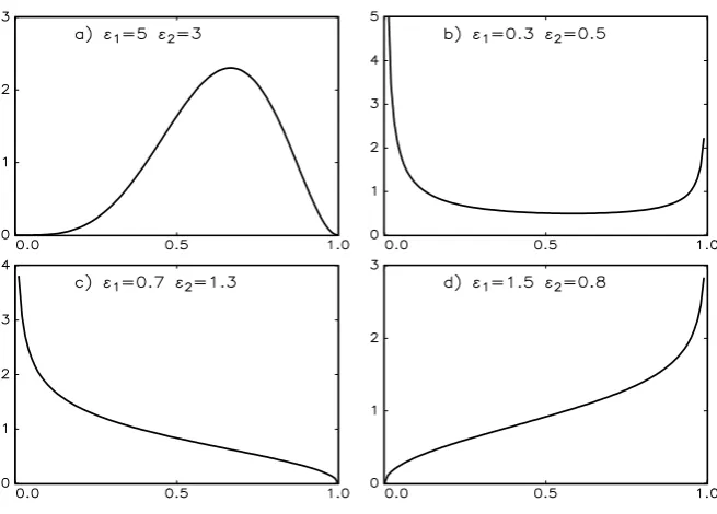
Figure 1 illustrates the flexibility in the shape of the beta distribution, with unimodal and bimodal cases similar to the symmetric case (11) in the top panel (a,b), but also including monotonically increasing or decreasing cases in situations where agents have a strong idiosyncratic signal in one direction, yet still exhibit a relatively pronounced herding tendency relative to the other state, i.e. a1/b <1< a2/b or vice versa, as shown in the bottom panel (c,d).

Figure 1: Beta distribution for various parameter combinations.

its parsimony, the model produces a wide range of qualitatively different statistical equilibria, including endogenous cycles in expectations caused by herding or imitation, but also equilibria where the vast majority of agents ‘learns a correct state’ in spite of being surrounded by noise that is created through the social interaction with neighboring agents. The qualitative fea-tures of the process are also parsimoniously summarized by the ratios (12) or (15), putting us in a position to isolate behavioral aspects from the question whether it is feasible to identify the communication or network structure among agents from survey data.

social interactions or model-consistent beliefs.

3

Random Benchmark and Simulation

We start with a thought experiment, putting ourselves in the position of an omniscient modeler (OM) who chooses a particular behavioral setup and net-work structure for the model in Section 2. Utilizing the individual transition rates (1) and (2), the OM simulates and records the time evolution of beliefs for allN agents in the system. Afterwards, the OM presents us with data on the individual histories of agents’ beliefs (or output for short), from which we have to determine the network structure among agents based on correlations in the time evolution of their beliefs.

In actual data on survey expectations, with typically two to three hundred agents reporting monthly beliefs over roughly two hundred periods, we have no intrinsic knowledge of the network structure whatsoever. So to make life easier for us, the OM even informs us of the exact number Di of neighbors

for each agent i = 1, . . . , N. We then compute the Di highest correlations

for each agent from the output and report it back to the OM as our best guess of the network structure in the output. In return, the OM checks our guesses against the actual identity of neighbors and reveals the fraction of correctly identified neighbors to us. The central question is: how many of the

Di neighbors do we expect to guess correctly by pure chance, i.e.irrespective

of the correlation among responses? This establishes a random benchmark against which we have to judge the success of correlation-based procedures.2

In order to explain the random benchmark, it is instructive to consider a simple urn model. Let us drawd(read: Di) colored balls without replacement

from an urn containing a total of N balls, m of which are white (read: the true neighbors of agent i). The probability of drawing k ≤m white balls in

2

Instead of considering the timet_{correlation, we have conducted the subsequent}

d draws from a total of N balls is given by the hypergeometric distribution

P[k] =

m k

N−m d−k

N d

, (16)

where the notation on the right hand side refers to binomial coefficients. In other words, (16) characterizes the distribution of the number of white balls drawn from the urn in dextractions. The mean value of the hypergeometric distribution is

E[k] = dm

N , (17)

from which we can compute the random benchmark since d=m in our OM setup.3 _{The standard deviation of the hypergeometric distribution is}

σ[k] =

s

dm(N −m)(N −d)

(N −1)N2 . (18)

To keep our simulations in line with available survey data (for instance from the ZEW for German ‘financial experts’, or from the FRB Philadelphia for US ‘professional forecasters’), we set the number of agents to N = 250; the available length of periods for individual agent IDs is on average between one and two hundred, while the number of questions per survey is typically between thirty and sixty. It will be a sobering experience to recall these figures when we present the simulation results.

3.1

Simulation setup

Regarding the network structure in our simulations, we consider three proto-typical setups: random graphs in the Erd¨os-Renyi tradition, scale-free net-works in the Barabasi-Albert tradition, and regular lattice structures.4 To keep matters simple, we set the number of neighbors equal to twenty in the

3

Notice that choosing a different number of extractions does not change any of the qualitative features in the following results, yet the approach immediately translates into quantitative prescriptions for measuring different benchmarks.

4

lattice, and tune the parameters of the scale-free and random networks such that we obtain adjacency matrices with an average number of twenty neigh-bors as well.5 _{Given these numbers and (17) and (18), it is straightforward}

to compute that the fraction of correct answers we would expect purely by chance corresponds to E[k] = 1.6 with σ[k] = 1.16, or normalized with re-spect to the number of extractions E[k]/d= 0.08 and σ[k]/d= 0.058.

In the subsequent figures, we use the mean plus one standard deviation,

E[k] +σ[k] = 2.76, to illustrate the statistical significance of the OM experi-ment. We can compute the probability of such an event from the cumulative hypergeometric distribution: since the hypergeometric distribution is defined for positive integer values of k, we have to consider P(k ≤ 2) = 0.79 and

P(k ≤3) = 0.94. Hence the range 0 < E[k] +σ[k]<3 delivers a rather con-servative confidence interval in accord with the usual econometric standards. In line with (1), (2) and (13), the OM implements the transition proba-bilities φi for each agent i as

φ(_i±) =ρ_i(±) ∆t= [a(1,2)+bD(

∓)

i ] ∆t with ∆t= 1/(amax+bN), (19)

where the notation D_i(∓) refers to the number of i-neighbors that are in the opposite state, and amax = max{a1, a2}. The choice of ∆t ensures both that

0< φi ≤1 and that all agents act on the same time scale.

The OM then confronts us with the output of theN time series of agents’ beliefs, from which we computeN(N−1)/2 correlation coefficients. For every

i, the OM also informs us of the actual numberDi of neighbors, and in turn

we extract theDi highest correlation coefficients from the output. Intuitively

assuming that the highest correlation coefficients correspond to the neighbors of agenti, we construct the adjacency matrix of the agent network and report it to the OM who compares it with the actual adjacency matrix, and informs us of the fraction of correctly identified neighbors for each i. To aggregate and visualize the results for each of the following three scenarios, we average

5

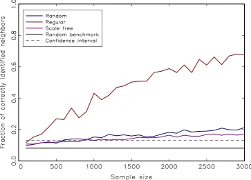
Figure 2: Average fraction of correctly identified neighbors vs length of in-dividual agents’ time series for a single question. We chose a bimodal simu-lation setup with parameters ε1 =ε2 =.5 and b= 1, i.e. a strong behavioral

component relative to symmetric exogenous signals in either direction.

the correctly identified percentages for each agent over the entire pool of agents.

The following scenarios basically consider in how far we can recover the correct network structure (i) depending on the length of agent histories and (ii) depending on the number of simultaneous survey answers per agent, i.e.

Figure 3: Average fraction of correctly identified neighbors vs length of in-dividual agents’ time series for a single question. Here we chose a unimodal simulation setup with parameters ε1 = ε2 = 2 and b = 1, i.e. a relatively

strong exogenous signal compared to the behavioral component.

3.2

Scenario I: Single indicator histories

Suppose when agents answer questions regarding rather distant areas of ex-pertise (e.g.international equity indices vs bonds vs GDP growth vs inflation etc.), they utilize different networks to form their expectations. So if we use histories for a single indicator in the OM experiment, what is the required number of observations per agent (or sample size for short) that is necessary to discriminate between some genuine network structure and random noise?

they are all arranged in a regular lattice. Regular networks, however, are the least suitable representation of observed social networks, which tend to interpolate between random and scale-free structures (see, e.g., Newman, 2003, and the references therein). This is also the reason why we focus our attention on random graphs in the coming scenarios.

As one would intuitively suspect, the identification of interaction effects is somewhat facilitated in the bimodal case, i.e. when herding or imitation dominate the expectations formation process. According to Figures 2 and 3, however, this aspect has merely second-order effects. Up to a sample size of around one thousand periods, we are not able to distinguish between noise and network effects if our knowledge is restricted to the time evolution of univariate histories. Hence this also implies that we do not have a sufficient number of empirical survey data at our disposal to reliably identify the social interaction component. Viewed from this perspective, any cluster we identify based on the cross-correlations of answers is essentially pure noise. If we consider the confidence interval in Figures 2 and 3, the first scenario suggests that it is entirely unrealistic to identify even a rudimentary communication structure unless we increase the frequency of survey responses by one order of magnitude, i.e.from monthly to roughly twice per week. In addition, if we are indeed facing irregular network structures, the length of single indicator histories that is necessary to correctly identify about half the neighbors turns out to be two orders of magnitude larger than empirical sample sizes.6

3.3

Scenario II: Multiple indicator histories

Can we improve the identification of communication structures if we make the strong assumption that behavioral parameters in the expectations for-mation process of agents do not change across multiple questions, and that their network structure remains unchanged as well? And how many questions would be necessary in that case? To tackle this issue, we keep the parame-terizations of the previous scenario and simulate the expectations formation process on a random network, fixing the length of single question histories

6

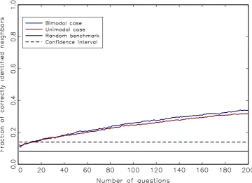
Figure 4: Increasing the number of questions and averaging over them im-proves the identification of interaction effects compared to the previous uni-variate scenario. The model parameterizations remain the same as before, and we utilize a random network whose structure remains fixed as well. The underlying univariate responses have a length of two hundred periods.

to two hundred while successively increasing the number of questions. Es-sentially, this means that the correlation coefficients are averaged both over agents and over questions. To operationalize this procedure, we fix the pa-rameterization and underlying network structure of social interactions and run K independent simulations of the model for two hundred periods. For each single run of length two hundred, we perform the estimation procedure outlined in the previous scenario, and then average over the K questions.

feature of this scenario is that the rate at which we discover actual links is markedly higher than in the univariate case. On the downside, however, the overall accuracy of the correlation-based procedure remains low. Keeping in mind that the empirical volume of survey coverage includes roughly thirty to sixty questions, correlation-based estimates of the interaction structure are almost not significantly different from pure noise, and certainly very low to begin with: we recover merely twenty percent of the actual network struc-ture, and the fraction of correctly identified neighbors increases very slowly with the number of questions.

3.4

Scenario III: Exogenously switching signal

In both of the preceding scenarios we have assumed that all agents have a strictly positive interaction parameter, which we conveniently set to b = 1. But what happens if some agents are not socially interacting at all (b = 0) and instead form model-consistent beliefs from exogenous signals a1, a2 that we

can think of as transmitting the correct state of the world? In principle, these ‘rational’ agents should exhibit highly correlated responses over time if the exogenous signal is sufficiently strong relative to the interaction parameter. If the state of the world does not change over time, the rational agents will all converge to the correct state, making it almost trivial to identify them from correlation-based procedures. In order to maintain an empirically more relevant scenario, we thus assume that the correct state of the world changes every now and then, i.e. the parameters a1, a2 are no longer constant but

change over time.7

In this scenario, we keep the total number of agents at N = 250 in our simulations, and the underlying network remains a random graph with an average degree of twenty neighbors. The values of ˜a1 = ˜a2 = ˜b = 1 are

constant over time for the majority ˜N = 200 of agents, while a smaller group of fifty ‘rational’ agents exhibits time-varying idiosyncratic coefficients, say

a1(t) anda2(t), which essentially measure the speed at which rational agents

7

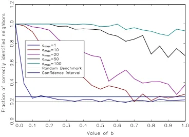
Figure 5: Fraction of correctly identified rational agents who follow a time-varying exogenous signal that is increasingly biased in either direction (de-noted by an increasing value of amax) vs their interaction strength b. At low

values of b, the identification generally performs very well, while higher val-ues of b might prevent a reliable detection, depending on the relative value of amax.

learn the true state of the world. The time-varying coefficients take on values in the set {1, amax}, where amax = max{a1(t), a2(t)}. Suppose for instance

that amax = 10 and that the currently ‘true’ state is such thata1(0) = 1 and

a2(0) = 10, i.e. we are in an optimistic regime today. When the true state

changes to pessimism, say in period τ, the parameters change toa1(τ) = 10

and a2(τ) = 1. As far as the switching probability in our simulations is

concerned, we assume that the probability to switch is five percent, drawn randomly from a uniform distribution. In other words, an exogenous switch in the signal occurs on average every twenty months in our simulations.

certainly does in reality. (Notice that we have to adapt the error band since nowd=m= 50.) None the less, we would expect the value ofb to also have an influence on our ability to identify the rational agents: when b increases, the noise generated through the social interactions with the other agents should make it more difficult to identify rational agents correctly. On the other hand, when rational agents are not part of the social network (b = 0), and thus do not take possibly non-rational opinons into account, it should become easier to correctly identify them with correlation-based procedures.

Figure 5 plots the fraction of correctly identified rational agents for a given amax when the interaction parameter b takes on values in [0,1]. The

different plots in Figure 5 refer to increasing values ofamaxin the simulations.

As expected, our ability to correctly identify the group of rational agents depends inversely on their interaction parameter b, possibly approaching the noise level asb approaches the value common to the other ˜N agents. On the other hand, when b approaches zero, we are in an increasingly comfortable position regarding the identification of rational agents. Finally, the faster the signal processing ability amax, the easier it becomes to correctly identify the

group of rational agents, asymptotically reaching the value of one hundred percent independently of b.

4

Discussion and Conclusions

All computations in the preceding scenarios have been performed under the assumption that the OM informs us of the actual number Di of neighbors

for each agent. Clearly, this is a most unrealistic assumption in the context of empirical applications to survey data, where we simply have no way of knowing whether agents interact socially in the first place, much less to whom they are linked to in case they do. Viewed from this perspective, our results are if anything overly optimistic to begin with.

the identification of network structure through an appropriate combination of b and a time-varying exogenous signal amax. The other side of that coin

is that we have no way of distinguishing between interaction effects and model-consistent beliefs, even if we identify relatively strong patterns in the correlations of a subset of agents.

Ultimately, these results suggest that existing survey data cannot facil-itate our understanding of the process of expectations formation, which is particularly troubling in light of its central importance for modern macroe-conomic theory. To end on a more constructive note, we would like to point out once more that our thought experiment presumed that we merely have data on the time evolution of agents’ beliefs. In order to investigate whether interaction effects are indeed present in the data, it would be enormously helpful if surveys contained questions that refer directly to the presence of interaction effects.

References

S. Alfarano and M. Milakovi´c. Network structure andN-dependence in agent-based herding models. Journal of Economic Dynamics and Control, 33: 78–92, 2009.

S. Alfarano, T. Lux, and F. Wagner. Estimation of agent-based models: The case of an asymmetric herding model. Computational Economics, 26: 19–49, 2005.

S. Alfarano, T. Lux, and F. Wagner. Time-variation of higher moments in a financial market with heterogeneous agents: An analytical approach.

Journal of Economic Dynamics and Control, 32:101–136, 2008.

M. Aoki. New Approaches to Macroeconomic Modeling. Cambridge Univer-sity Press, Cambridge, UK, 1998.

W. A. Brock and S. N. Durlauf. Discrete choice with social interactions.

Review of Economic Studies, 68(2):235–60, 2001.

C. D. Carroll. Macroeconomic expectations of households and professional forecasters. Quarterly Journal of Economics, 118(1):269–298, 2003.

M. P. Clements. Explanations of the inconsistencies in survey respondents’ forecasts. European Economic Review, 54(4):536–549, 2010.

O. Coibion and Y. Gorodnichenko. What can survey forecasts tell us about informational rigidities? NBER Working Paper 14586, National Bureau of Economic Research, December 2008.

M. Del Negro and S. Eusepi. Modeling observed inflation expectations. mimeo, Federal Reserve Bank of New York, 2009.

G. Evans and S. Honkapohja. Learning and Expectations in Macroeconomics. Princeton University Press, Princeton, 2001.

B. Flieth and J. Foster. Interactive expectations. Journal of Evolutionary Economics, 12(4):375–395, 2002.

C. H. Hommes. The heterogeneous expectations hypothesis: Some evidence from the lab. mimeo, University of Amsterdam, Netherlands, 2010.

A. Kirman. Epidemics of opinion and speculative bubbles in financial mar-kets. In M. P. Taylor, editor,Money and Financial Markets, pages 354–368. Blackwell, Cambridge, 1991.

A. Kirman. Ants, rationality, and recruitment. Quarterly Journal of Eco-nomics, 108:137–156, 1993.

M. Lines and F. Westerhoff. Inflation expectations and macroeconomic dy-namics: The case of rational versus extrapolative expectations. Journal of Economic Dynamics and Control, 34:246–257, 2010.

N. G. Mankiw and R. Reis. Sticky information versus sticky prices: A pro-posal to replace the New Keynesian Phillips curve. Quarterly Journal of Economics, 117(4):1295–1328, 2002.

N. G. Mankiw, R. Reis, and J. Wolfers. Disagreement about inflation ex-pectations. In NBER Macroeconomics Annual 2003, volume 18, pages 209–270, Cambridge, July 2004. MIT Press.

F. Milani. Expectation shocks and learning as drivers of the business cy-cle. CEPR Discussion Paper 7743, Centre for Economic Policy Research, March 2010.

M. Newman. The structure and function of complex networks. SIAM Review, 45:167–256, 2003.

M. H. Pesaran and M. Weale. Survey expectations. In G. Elliott, C. Granger, and A. Timmermann, editors, Handbook of Economic Forecasting, vol-ume 1, chapter 14, pages 715–776. Elsevier, 2006.

C. A. Sims. Implications of rational inattention. Journal of Monetary Eco-nomics, 50(3):665–690, 2003.

W. Weidlich. Sociodynamics: A Systemic Approach to Mathematical Mod-elling in the Social Sciences. Dover, New York, 2006.

W. Weidlich and G. Haag.Concepts and Methods of a Quantitative Sociology. Springer, Berlin, 1983.