Journal of Chemical and Pharmaceutical Research, 2015, 7(3):2541-2549
Research Article
CODEN(USA) : JCPRC5ISSN : 0975-7384Design and performance analysis of delay tolerance network secure routing in
a harsh wild scenario
Zhou Honghai* and Jin Zhihao
Nanjing University of Science and Technology, China
_____________________________________________________________________________________________
ABSTRACT
Based on the research of the DTN secure routing in a harsh wild scenario, a novel DTN secure routing method was proposed, in which G/G/1 model and Chebyshev inequality were used in modeling and figuring out the key parameters. After that was a simulation experiment of the whole DTN process under ONES simulation tools, and the experimental data was compared with the expected data to confirm the key factors that are affecting system transmission efficiency.
Key words: Delay Tolerant Network; harsh wild scenario; queuing theory
_____________________________________________________________________________________________
INTRODUCTION
Harsh wild Scenario is a special network application structure which is emerged as the demands of military and expedition nowadays. Complex environment includes local high density of fire, signal masking, extreme weather events and some other harsh environment that affect secure communication. In these conditions, wireless communication nodes will be damaged and cause a crash in network link, so combat units cannot communicate in security directly .Therefore, a DTN routing is needed in order to realize efficient transmission under some degree of delay tolerance. Research institutions at home and abroad have proposed many DTN scenarios based on DTN special transmission method. For example, NASA[1] proposed Periodic connection with satellite network , Nikolaos et al [3]proposed Delay tolerant bulk data transfer on the Internet ,etc. But the DTN secure routing research in the scenario of harsh wild is not mature.
In a harsh wild scenario, because of resource starvation in combat radius, participants ,who were divided into several combat groups and scattered to different combat areas ,could not communicate with each other in real time. And as the secrecy and anti-reconnaissance of a military action, every group took action without carrying a long-distance mobile device and was not visible to others. So other methods, like semaphores, were unworkable. As a result, every group didn’t share an end-to-end secure link, so a DTN network has to be formed to transfer message in non-real time. And every group should equip a mobile proxy node which should meets:
1. Could carry several pieces of datagram message and understand the delivery target and corresponding route in order to reach the target.
2. After the delivery, proxy node could go back to data source(the corresponding combat group) 3. Could finish 1 and 2 within the allotted time.
4. Node could be a robot, a remote control device or a combat participant.
proxy node is shared by all nodes in the network and plays the messenger role in secure communication network.
Although harsh wild scenario DTN network (for harsh wild scenario DTN hereafter) belongs to the DTN routing with auxiliary nodes theoretically. But unlike other routing of this category, every mobile proxy node in this scenario has a fixed and unique affiliation to the corresponding data source node, to avoid competition for network resources and transmission rate decrease caused by demand imbalance between data source and sharing mobile proxy node. If every data source owns an assigned mobile secure communication node, we can focus most of the energy on the performance improvement of a single node without considering the resource contention between data source nodes. Harras and Almeroth el al [4] proposed to apply mobile proxy node in a similar scenario. But in the model Harras built, mobile proxy node delivers message to only one ultimate destination node each time, instead of multi-targets delivering in order. Harsh wild scenario DTN overcomes the above shortcomings.
The reminder of this paper is organized as follows. Section Ⅱ introduces a harsh wild scenario DTN network
model, of which queuing theory is used to do performance analysis. SectionⅢ simulates the harsh wild scenario
DTN model, and the experimental results obtained will be compared with theoretical data.
ⅡHARSH WILD SCENARIO DTN MODEL
In a harsh wild scenario DTN network with n nodes, we assign one node as data source node, while other nodes are all participant nodes. To simplify the analysis process, we assume that source node generates messages with Poisson
distribution of which the average value is λ, and the messages are put into a FIFO queue. When the mobile proxy
node leaves the source node, it will get fixed pieces of messages to its own message queue in order (as shown in Fig. 1, ultimate destination nodes of the 6 pieces of messages are 1,3,4,5,6,9 respectively). The proxy node moves to each destination node in turn at a constant velocity v and deliver message to each corresponding destination node. After all the delivery is done, the proxy node will go back to the source node. All participant nodes are distributed on an arc of length 1 whose circle center is the data source, so the distance to every participant node is the same after proxy node departuring from the data source.
Fig. 1: A simple illustration of harsh wild scenario DTN
When data source generates a piece of message, it will randomly choose one participant node as a destination. A successful delivery depends (1) message reached destination node successfully.(2)transmission time should be within expiration time ,or the message will be dropped.
When belonging proxy node is filled up with the destination information, it will start transmission at the leftmost destination node and move to the next in a clockwise.
______________________________________________________________________________
a mobile proxy node has one bulk service queue which satisfied the feature of G/G/1 model with a capacity s (all the calculation and analysis in the rest of this paper are based on this assumption). According to queuing theory, in order to deduce the delay and arrival rate, we should figure out the service time and waiting time of one piece of message first, which are also relevant with the service time and waiting time of bulk data.
BULK DATA SERVICE TIME X
In harsh wild scenario DTN model, bulk data service time is the interval between a proxy node departuring from the data source and it coming back to the data source. i.e. the time interval that data transmission task is completely done. Obviously that delay is determined by the data service time, so the expectation and variance of service time are needed to help figuring out the expectation and variance of message delay.
First of all, a mobile proxy node is about to leave data source to reach k (k ≥ 1) different destination nodes with a
batch of messages. As mentioned before, n participant nodes are distributed on an arc of length 1 , and k destination nodes is selected from n participant nodes according to probability. So here is a conclusion that k destination nodes are scattered randomly on the arc of length 1.
, … are kvalues distributed randomly in the interval [0,1] with an increasing order. (1 ≤ ≤ )represents
the distance from the leftmost participant node to the ith destination node, that is , stands the leftmost destination
node, while stands the rightmost. - shows the max transmission distanceof exponent data node on the arc.
Let F(x) and f(x)be the cumulative distribution function and probability density function of . As obeying
the uniform distribution, obviously, F(x) = x,f(x) = 1.And we can have the probability density function of :
( )= ( ) − 1 ( )− 1 1 − ( ) = − 1− 1 (1 − ) (1)
If radius r of the arc is a constant, the distance that proxy node covers each time isL = 2 + ( )− ( ). From Eq.1:
( )
!!!!! = "$ ( )( ) # = "$ # = /( + 1) (2)
( )
!!!!! = "$ ( )( ) # = " (1 − )$ # = 1/( + 1) (3)
( )
!!!!!!! = "$ # = /( + 2) (4)
( )
!!!!!!! = " −( − 1)$ # = 2/[( + 1) ( + 2)] (5)
Therefore, the average transmission distance of the exponent data node
L
kequals:(!!! = 2 + !!!!! −( ) !!!!! = 2 +( ) ) − ) = 2 + ) (6)
Let * be the time that mobile proxy node need to finish k transmission tasks. When proxy node get a velocity v,
here is:
*!!!! =+!!!!,
- = .
- +( ) )- (7)
The secondary moment of * is:
φk2
!!!!!=L!!!!k2 v2 1 =4r2
v2 +(k+1)v4r(k-1)2+ k 3-3k+2
v2(k+1)2(k+2) (8)
Besides the mentioned results above, a function6( ) is also needed to select k nodes from n participant nodes (as
destination nodes to receive s messages). 6( )is relevant with 2 components:
7( ):The probability that k participant nodes are selected from n nodes as potential destination nodes to receive s
messages.
ℎ( ):The probability that k nodes given happen to be the destination nodes to receive s messages .Obviously:
6( ) = 7( ) × ℎ( ) (9)
7( ) = : × ; < (10)
=(>, ), the number of methods that could divide s elements into k non-empty subsets, is needed to confirm h(k).
=(>, ) = !∑ (−1) B CDED<
BF (=(>, ) regardless of the order) (11)
As ℎ( ) =G(<, )× !H ,
ℎ( ) =G(<, )× !H = ∑ (−1)BF BCDE B < (12)
After calculating 7( )and ℎ( ), the expectation of bulk data service time X is confirmed as follows :
! = ∑ *!!!! ∗ 6( )<
F (13)
Similarly, the secondary moment of X is calculated as follows:
2 2
1
* ( )
S
k k
X
ϕ
p k
=
=
∑
(14)
And the variance of the bulk data service time X is δ K= !!!! − !
BULK SERVICE WAITING TIME W
Bulk service waiting time shows the time interval that from message m created by data source being inserted into service queue with capacity s, to proxy node being filled up and departuring from the data source. The queue service
model in harsh wild scenario DTN fits well with G/G/1 queue model. In G/G/1 model,
λ
is described as theaverage arrival rate of the task and the average value of task waiting time Wis :
LM =NOP)NOQR̅( T))(R̅)O( T)O−U!!!OU̅ (15)
In Eq.15 , t and VRare expectation and variance of the interarrival time of bulk data groups. According to G/G/1
model,W̅=>YX,VR= > XY .And Z = X ! >Y , where Z is system utilization. Variable I is the queue service idle time (i.e.
the time interval that the number of messages is less than s) and[̅ = > XY ,[M = (> + > ) XY . And then :
LM =T(<T <) )\( ]) + <( T)\NO^ (16)
The secondary moment of W can be confirmed then:
L
!!!!! =<( T[ \_M <( T)])
\O (17)
When the expectation and secondary moment of W were confirmed, the variance of W can be obtained:
σ a=<( T[ \_M <( T)])\O − LM (18)
SINGLE MESSAGE SERVICE TIME X’
In harsh wild scenario DTN model, as part of the message delay, the definition of single message service time X’ is similar to bulk data service time X: the time that from single piece of message departuring from the queue and being taken by proxy node, to that message arriving at the destination node.
As the destination node of the single message is selected randomly from k destination nodes, the expectation of this bulk data service time in G/G/1 queue is:
______________________________________________________________________________
Its secondary moment is:
b!!!! = ∑ ( +!!!!!!!!!!!!!!!!!!!!!!/d(c)− ( )) (20)
According to the concept of order statistics, we can obtain:
(c)
!!!!! = "$ ( )( ) # = − 1 ∑− 1 e− ( )
f
g) )
gF$ (21)
(c)
!!!!!! = "$ ( )( ) # = − 1 ∑− 1 e− ( )
f
g) )
gF$ (22)
Taken together, the expectation of single message service time is:
h
!!! = ∑ b × 6( )<
F (23)
The secondary moment is:
′
!!!! = ∑ b!!!!! × 6( )<
F (24)
The variance is:
σ K‘= ′!!!! − ′M (25)
SINGLE MESSAGE WAITING TIME W’
Single message waiting time W’ means the time that from proxy node taking one piece of message from data source
node to delivering it to the destination node successfully. If the interval kis defined as the time that from the first
piece of message being successfully delivered to the last message being able to deliver, then we have Lh= k + L.
In order to get W’, kis supposed to be calculated as W is known. As message waiting process shown in Fig. 2 , e (1 ≤ i ≤ s) represents the ith message in the proxy node queue, ηrepresents the arrival interval between e
ande. e$is defined as the last piece of message inserted into the message queue before proxy node departuring. In
harsh wild scenario DTN model, η ,η ….η<are random variables obeying independent and identically exponential
distribution, so ηcM = 1/X,σ op= 1/X .Assume thatkpequals the arrival interval between e ande<, thenk =
q) +q) + ⋯ +q<.The expectation of kp is:
kM =c ηc)!!!!!!!!!!!!!!!!!!!!!!!!!!! = (s − i)+ηc) + ⋯ +η< η! = (> − )/X (26)
Fig. 2: Message waiting process sketch
The secondary moment is:
k!!! = (!!!!!!!!!!!!!!!!!!!!!!!!!!!!!! =ηc) +ηc) + ⋯ +η<) <O)< ( <) ) )\O O (27)
k̅ =<∑ k<F Mc=<\ (28)
The secondary moment of k is:
k!!! = ∑ s(k | = )u( = )<
F =<∑ k<F !!!!c = −<)\O+<\O∑<F (29)
The variance of k is:
σ v= k!!! − k̅ = −G
O)w
x\O +<\O∑<F (30)
Askand bulk data waiting time W are independent, the expectation of single message waiting time Lhequals the sum of both expectations and variance is the sum of both variance.
From 2.1 to 2.4 ,this paper described in detail the calculating method of the process variables that relevant with message delay calculating.2.5 and 2.6 will figure out the message delay and message arrival rate from the results above.
MESSAGE DELAY
In harsh wild scenario DTN, according to the queuing theory, message delay T means the time that single piece of message stays in system.
b = L’+ ‘
The expectation of b is:
b! = L!!!!!!!!!! = L′h+ ′ !!!! + ′M (32)
As the single message waiting time and single message service time are independent, then:
Vz =V_ + VK (33)
MESSAGE ARRIVAL RATE
To figure out the margin value of the message arrival rate, T is plugged into Chebyshev inequality, so:
P[T − b! ≥ ε] ≤ P[|T − b!| ≥ ε] ≤N~O
•O (34)
Through derivation:
P[T ≤ ε + b!] ≥ 1 −N~O
•O (35)
Let constant
Γ
be the expiration time of all messages, then the probability that a piece of message could be delivered to the destination node within expiration time is:P[T ≤ τ] ≥ 1 − N~O
(• z!)O (36)
Above all, the message delay and message arrival rate can be confirmed. And the harsh wild scenario DTN service model has been established. Next section, a system simulation will be conducted to analyze the performance of the harsh wild scenario DTN through comparing the experimental results and theoretical results.
ⅢSYSTEM SIMULATION
______________________________________________________________________________
Fig. 3: the harsh wild scenario DTN simulation process
The experiment parameters are set as follows:
(1)Experiment duration: 43200ms, which represents 43200s in reality, i.e. 12 hours.
(2)Mobile proxy node moving velocity: 1.5 length unit/ms
(3)Number of source nodes:1 , number of mobile proxy nodes:1 ,number of participant nodes : 15
(4)Arc radius: 1/πlength unit
(5)Participant node type: low-power consuming node. Source node and mobile proxy node type: high-power node
with wider range of secure communication.
(6)The experimental result would be stored in jbdtn_scenario_MessageDeliveryReport .
In harsh wild scenario DTN simulation experiment, only node moving velocity v and queue size s are artificial
controlled. From modeling in sectionⅡ, message transfer rate is fundamentally proportional to velocity v.
But the influence of the variation of queue size s of the system is not yet clear. We need regard v as a fixed constant to analyze the experimental results.
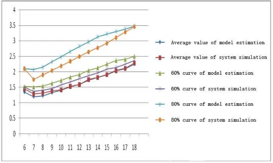
Fig.4 shows the theoretical data and simulated data with different queue size s. To provide a more direct result, a systematic sampling percentage is obtained through statistics of 200 trials results when analyzing. 80% curve or 60% curve represents that 80% or 60% sample values in model estimation or simulation are less than the message delay at the corresponding queue size s. The average arrival rateλ of the task is 5,10, respectively, and whenλ takes different value, the changing tendency of the curve is basically accorded. Also, the simulated average curve is basically agreed with the model estimated curve .This indicates that harsh wild scenario DTN model is feasible in both principle and reality. (in addition, the corresponding systematic sampling percentage difference of model estimation and simulation is less than 5%.That is acceptable.)
(b)λ=10,s=13 30 x axis represents s,y axis represents message delay
[image:8.595.116.504.308.449.2]Fig. 4: the changing curves of message delay with different λ and s
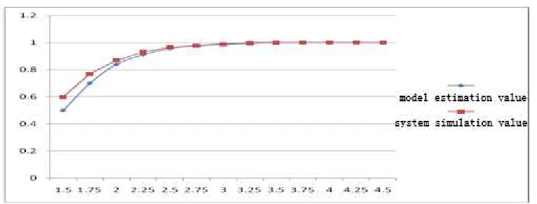
Fig. 5 shows the changing curve of system message arrival rate with different 2 sets of s andλ. The horizontal axis
shows the max system message transmission time .Through observation, the difference between model estimation values and simulation results is negligible.
(a) λ=5,s=7 x-axis represents the max message transmission time, y-axis represents message arrival rate
(b) λ=10, s=13x-axis represents the max message transmission time, y-axis represents message arrival rate
Fig. 5: the changing curves of system message arrival rate with differentλ and s
By comparing the curves in Fig. 4, there is an only queue size s that could lead to the shortest system message delay.
That is, when message arrival rateλ is unknown, harsh wild scenario DTN model can be corrected and optimized by
confirming s. Moreover, as shown in Fig. 4, whenλ is 5 or 10, the corresponding curves share the same shortest delay s (λ=5,s=7;λ=10,s=14). And the shortest message delay corresponds to the smallest system message arrival
rate. According to Section Ⅱ, system message arrival rate is relevant with both the variance and expectation of the
delay. Fig. 6 shows the arrival rate – delay curve atλ=5,s=6~25 , and the horizontal axis is message delay while the
[image:8.595.116.499.478.624.2]______________________________________________________________________________
message delay.
λ=5, s=6 30 x-axis represents the message delay, y-axis represents message arrival rate
Fig. 6: The system message arrival rate-message delay curve
In summary, to reach the expected system message arrival rate in harsh wild DTN model, a shortest message delay is necessary which can be confirmed by selecting appropriate queue size s. That is, an appropriate queue size s will help to reach the most ideal delivery efficiency in harsh wild scenario DTN.
CONCLUSION
In this paper, we proposed a novel DTN secure routing method based on the research of the DTN secure routing in a harsh wild scenario. In the proposed method, G/G/1 queue model and Chebyshev inequality were used in modeling and figuring out the key parameters .After that was a simulation experiment of the whole DTN process under ONES simulation tools, and the experimental data was matched with the expected data. At last we draw the conclusion that message queue size s decides the optimal transfer efficiency of DTN in a harsh wild scenario.
REFERENCES
[1]Nichols K, Holbrook M, Pitts RL.Dtn implementation and utilization options on the international space
station.2012-bioserve.colorado.edu
[2]Qianmu L. An International Interdisciplinary Journal,2011, vol. 14, no. 3, :731-738.
[3]Laoutaris N, Smaragdakis G, Rodriguez P, Sundaram R. Delay tolerant bulk data transfers on the internet. In
proceeding of: Proceedings of the Eleventh International Joint Conference on Measurement and Modeling of Computer Systems, SIGMETRICS/Performance 2009, Seattle, WA, USA, June 15-19, 2009
[4]Harras K.A, Almeroth KC.Inter-Regional Messenger Scheduling in Delay Tolerant Mobile Networks in
Proceedings of IEEE WoWMoM,2006
[5]Li Q M, Hou J, Qi Y, Zhang H. Disaster Advances, 2012,5(4):432-437.
[6]Li Q M, Zhang H. Information- an International Interdisciplinary Journal,2012,15(11):4677-4684.